
本篇的 Pandas 格式說明,可以想像成在 Python 中如何操作 Excel 表格,比如如何建立 Excel 表格,如何存檔讀檔,如何選取欄或列,如何計算。
Pandas 貓熊
pandas 是 Python 一個重要的數據分析套件,於2009年開源出來,以 numpy 為基本資料型態,再度創造另一種高效易用的資料格式(DataFrame),可以快速進行資料分析。
Pandas 的基本資料格式叫 DataFrame,簡稱 df。DataFrame 這名詞不好理解,一般教學也說不清楚,其實很簡單,只要把 DataFrame 想成是一張 Excel 工作表格即可。
Pandas 可以讀取 Excel 檔案產生 DataFrame 資料格式,DataFrame 也可以將裏面的資料存成 Excel 檔。學習 Pandas 就好像在學習怎麼用 Python 操作 Excel。
使用前, 必需先 pip install pandas, 記注意, 有加 “s” 喔
補充說明
標準正態分佈(Standard normal distribution) : 又稱為u分佈,是以0為均值、以1為標準差的正態分佈,記為N(0,1)
np.random.randn(4,3,2) : 產生三維的正態分佈亂數, 維度可以隨便增加, 也可以是一維
Pandas的資料結構
Series : 類似 Excel 表格,但只有一個欄位。有自已的索引, 也可以自行命名。
DataFrame : 類似 Excel 表格,可以有欄位名,而每列資料錄可以有索引。
Series
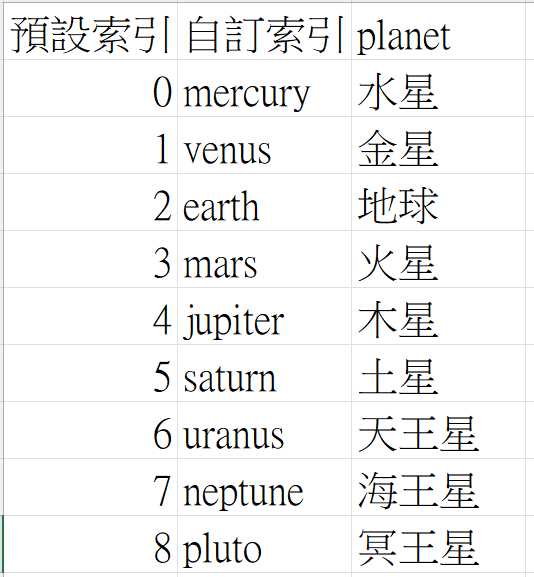
Series 其實只有一個欄位,但有多筆資料。每筆資料都可以自訂索引,如下圖。
Series的用途,除了可以使用索引指定資料外,也可以使用標籤來指定,比如 s[0],或 s[‘地址’]。
預設索引
產生Series的方式,可以使用 pd.Series([]), 將list或np.array([])或字典 資料傳入, 如下示範list及array的使用方式。
import pandas as pd
import numpy as np
s1=pd.Series([1,2,3,4,5])
print(s1)
print("s1[4]=%d " % s1[4])
s2=pd.Series(np.random.randint(0,3,5))
print(s2)
結果 :
0 1
1 2
2 3
3 4
4 5
dtype: int64
s1[4]=5
0 1
1 1
2 0
3 0
4 2
dtype: int32
自訂索引
Series 的自訂索引需在 Series 方法中加入 index 參數,index 可以為數字,也可以為字串。
當 index 為字串時,稱為標籤(Label),同時也會產生由 0 開始的索引。
當 index 為數字時,則只有索引,沒有標籤。
另外請注意一件事,index可以為list,亦可以為np 的陣列格式。
pd.Series([資料…], index=[索引…])
pd.Series([資料…], index=np.array([索引…]))
當有自訂標籤時,雖說也有索引,可以使用 s[4]這種寫法,但在新版的 Pandas 會出現如下警告
FutureWarning: Series.__getitem__ treating keys as positions is deprecated. In a future version, integer keys will always be treated as labels (consistent with DataFrame behavior). To access a value by position, use `ser.iloc[pos]`
這個警告是說 s[4] 這種寫法即將被拋棄,請改用 s.iloc[4],指定第 4 列的意思。
import pandas as pd
index=['mercury','venus','earth','mars','jupiter','saturn','uranus','neptune','pluto']
planet=['水星','金星','地球','火星','木星','土星','天王星','海王星','冥王星']
s=pd.Series(planet, index=index)
print(s)
print(f"s.iloc[4]={s.iloc[4]}")
print(f"s['jupiter']={s['jupiter']}")
結果 :
mercury     水星
venus       金星
earth       地球
mars        火星
jupiter     木星
saturn      土星
uranus     天王星
neptune    海王星
pluto      冥王星
dtype: object
s[4]=木星
s['jupiter']=木星
使用字典資料
Series 亦可使用字典產生,如下所示。
import pandas as pd
d={'name':'Thomas', 'sex':'female', 'age':50, 'phone':'0989889123'}
s=pd.Series(d)
print(s)

print('讀取值,可用如下三個方法,分別為索引,標籤,多索引list')
print(f'索引 : {s[0]}')
print(f'標籤 : {s["name"]}')
print(f'多索引 : \n{s[[0,1,2]]}')
print(f'多標籤 : \n{s[['name', 'sex']]}

結果 :
name Thomas
sex female
age 50
phone 0989889123
dtype: object
讀取值,可用如下三個方法,分別為索引,標籤,多索引list
索引 : Thomas
標籤 : Thomas
多索引 :
name Thomas
sex female
age 50
多標籤 :
name Thomas
sex female
dtype: object
上述 s[[0,1,2]] 看起來怪怪的,請記得最外面的 “[]” 是包含索引的符號,而裏面的 “[]” 則是 List。
s[ [list] ]
DataFrame
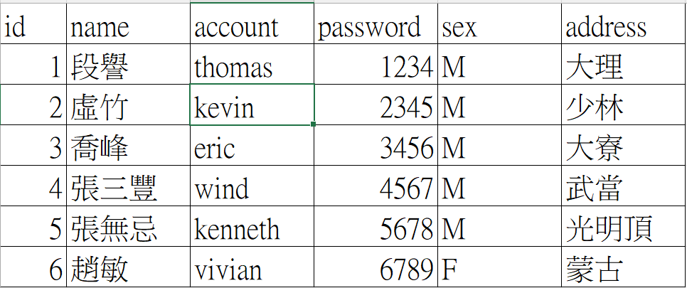
把 DataFrame 是具有多個欄位,多筆資料的 Excel 表格,每個欄位需有欄位名稱,每列需有索引,如下圖的資料所示。
產生DataFrame的方式,有三個要注意,一是欄位名稱,二是每個欄的內容值,三是每列的索引。
共有三種方式可以產生 DataFrame 格式,可以想像成有三種方式建立 Excel 表格,詳述如下。
第一種方式
以行為主,將每行的資料集合在List中,再將每個List 加入以欄位名為 key 的字典
import pandas as pd
data={
    'id': [1,2,3,4,5,6],
    'name' :  ['段譽','虛竹','喬峰','張三豐','張無忌','趙敏'],
    'account' : ['thomas','kevin','eric','wind','kenneth','vivian'],
    'password' : ['1234','2345','3456','4567','5678','6789'],
    'sex' : ['M','M','M','M','M','F'],
    'address': ['大理','少林','大寮','武當','光明頂','蒙古']
    }
df=pd.DataFrame(data)
print(df)
結果 :
   id name  account password sex address
0   1   段譽   thomas     1234   M      大理
1   2   虛竹    kevin     2345   M      少林
2   3   喬峰     eric     3456   M      大寮
3   4  張三豐     wind     4567   M      武當
4   5  張無忌  kenneth     5678   M     光明頂
5   6   趙敏   vivian     6789   F      蒙古
第二種方式
以列為主,每列以 {欄1:值1,欄2:值2, 欄3:值3} 的字典的方式形成,再將每列加入List中
import pandas as pd
data=[]
data.append({'id':1, 'name':'段譽', 'account':'thomas', 'password':'1234', 'sex':'M', 'address': '大理'})
data.append({'id':2, 'name':'虛竹', 'account':'kevin', 'password':'2345', 'sex':'M', 'address': '少林'})
data.append({'id':3, 'name':'喬峰', 'account':'eric', 'password':'3456', 'sex':'M', 'address': '大寮'})
data.append({'id':4, 'name':'張三豐', 'account':'wind', 'password':'4567', 'sex':'M', 'address': '武當'})
data.append({'id':5, 'name':'張無忌', 'account':'kenneth', 'password':'5678', 'sex':'M', 'address': '光明頂'})
data.append({'id':6, 'name':'趟敏', 'account':'vivian', 'password':'6789', 'sex':'F', 'address': '蒙古'})
df=pd.DataFrame(data)
print(df)
第三種方式
也是以列為主,每列的資料集合在 List 中,再將每列加入 List 中。最後指定columns
import pandas as pd
data=[]
data.append([1,'段譽','thomas','1234','M','大理'])
data.append([2, '虛竹', 'kevin', '2345', 'M', '少林'])
data.append([3, '喬峰', 'eric', '3456', 'M', '大寮'])
data.append([4, '張三豐', 'wind', '4567', 'M', '武當'])
data.append([5, '張無忌', 'kenneth', '5678', 'M', '光明頂'])
data.append([6, '趟敏', 'vivian', '6789', 'F', '蒙古'])
cols=['id','name','account','password','sex','address']
df=pd.DataFrame(data=data, columns=cols)
print(df)
完美列印DataFrame
如果想要完整列出所有資料,需在 print(df) 之前更改四個參數如下。
import pandas as pd
import plotly_express as px
df=px.data.gapminder().query('year==2007')
display=pd.options.display
display.max_columns=None
display.max_rows=None
display.width=None
display.max_colwidth=None
print(df)
Excel 計算
底下說明類似 Excel 的計算,假設有資料如下
    id          日期   姓名      帳號     薪資   時數
0    1  2025-05-05  羅凱莉   dodo133558  42800  1.0
1    2  2025-05-05  王駿晟    virage486  44000  1.5
2    3  2025-05-05  羅可杰     qwer0828  35700  3.0
3    4  2025-05-05  林意筑          lin  56200  3.0
4    5  2025-05-05   陳寬       Ronald  53300  3.0
5    6  2025-05-05  蔡長恩     pyro0329  41700  2.0
6    7  2025-05-05  蔡孟勳          sss  51900  4.0
7    8  2025-05-05  孫成岳        qwert  30900  2.0
8    9  2025-05-05  張凱富   heerochang  55500  5.0
取得資料
使用如下代碼取得上面的 df 資料
from G import G
import pandas as pd
display=pd.options.display
display.max_columns=None
display.max_rows=None
display.width=None
display.max_colwidth=None

conn, cursor=G.connect(
    host='localhost',
    user='帳號',
    password='密碼',
    database='cloud'
)
cursor.execute('select * from 加班資料')
columns=[d[0] for d in cursor.description]
rs=cursor.fetchall()
conn.close()
df=pd.DataFrame(data=rs, columns=columns)
#print(df)
#選取指定的欄位
df=df[["日期","姓名", "帳號",  "薪資", "時數",]]

#插入欄位
df.insert(len(df.columns), "加班費", 0)
取得欄位、欄數、列數
使用如下代碼取得欄位名及指定列數。
columns=df.columns.values.tolist()
print(columns)

#取得列數及欄數
rows=df.shape[0]
cols=df.shape[1]
print(f"共{rows}列, {cols}行")
指定列數
底下能將 2~32列的資料列出。
df=df.head(32).tail(30)
print(df)
重定 index
使用如下代碼重設 index
df.index=range(1, df.shape[0]+1)
print(df)
單欄位簡易計算
假設加班時薪是 100 元,底下是計算每個人的加班費
df['加班費']=df['時數']*100
print(df)
多欄位簡易計算
假設加班費是時薪的 1.33倍,
df['加班費']=df['薪資']/30/8*df['時數']*1.33
print(df)
多欄位複雜計算
複雜計算時需使用函數,此時需要使用 Lambda 語法
def overtime(x):
    if x<=2:
        pay=1.33*x
    else:
        pay=2*1.33+(x-2)*1.66
    return pay
df["加班費"]=df.apply(lambda row:row["薪資"]/30/8*overtime(row["時數"]),axis=1)
print(df)
plotly_express 練習資料
plotly_express是一個用於資料分析和資料圖表化的套件,在後續的視覺化中會有詳細的說明。
plotly_express 提供了 gapminder 資料表,其格式就是DataFrame。裏面的資料記錄了世界各國的國名,洲別,每年的人口平均壽命,人口數,國別簡碼及國別代碼。
在使用此範例前,請先 pip install plotly-express
底下的代碼會因欄及列的資料太多而無法完整列出,所以會有 … 只列出部分資料
import plotly_express as px
df = px.data.gapminder().query('year == 2007')
print(df)

結果 :
                 country continent  year  ...     gdpPercap  iso_alpha  iso_num
11           Afghanistan      Asia  2007  ...    974.580338        AFG        4
23               Albania    Europe  2007  ...   5937.029526        ALB        8
35               Algeria    Africa  2007  ...   6223.367465        DZA       12
47                Angola    Africa  2007  ...   4797.231267        AGO       24
59             Argentina  Americas  2007  ...  12779.379640        ARG       32
...                  ...       ...   ...  ...           ...        ...      ...
1655             Vietnam      Asia  2007  ...   2441.576404        VNM      704
1667  West Bank and Gaza      Asia  2007  ...   3025.349798        PSE      275
1679         Yemen, Rep.      Asia  2007  ...   2280.769906        YEM      887
1691              Zambia    Africa  2007  ...   1271.211593        ZMB      894
1703            Zimbabwe    Africa  2007  ...    469.709298        ZWE      716

[142 rows x 8 columns]
iloc
iloc 可以同時指定列及欄。 iloc 只能使用數字 list 或數字切片。
列切片
df.iloc[:5] 指定前 5 列,跟 df.loc[:5] 是同樣的功能
import pandas as pd
import plotly_express as px
dis=pd.options.display
dis.max_columns=None
dis.max_rows=None
dis.width=None
dis.max_colwidth=None
df=px.data.gapminder()
df=df.query("year==2007")
print(df[:5])
print(df.iloc[:5])
結果:
        country continent  year  lifeExp       pop     gdpPercap iso_alpha  iso_num
11  Afghanistan      Asia  2007   43.828  31889923    974.580338       AFG        4
23      Albania    Europe  2007   76.423   3600523   5937.029526       ALB        8
35      Algeria    Africa  2007   72.301  33333216   6223.367465       DZA       12
47       Angola    Africa  2007   42.731  12420476   4797.231267       AGO       24
59    Argentina  Americas  2007   75.320  40301927  12779.379640       ARG       32
指定特定列
df[] 只能使用切片,無法指定某幾列,但 df.iloc[[1,3,5,7]] 可以指定第 1,3,5,7 列
import pandas as pd
import plotly_express as px
dis=pd.options.display
dis.max_columns=None
dis.max_rows=None
dis.width=None
dis.max_colwidth=None
df=px.data.gapminder()
df=df.query("year==2007")
print(df.iloc[[1,3,5,7]])
結果:
      country continent  year  lifeExp       pop     gdpPercap iso_alpha  iso_num
23    Albania    Europe  2007   76.423   3600523   5937.029526       ALB        8
47     Angola    Africa  2007   42.731  12420476   4797.231267       AGO       24
71  Australia   Oceania  2007   81.235  20434176  34435.367440       AUS       36
95    Bahrain      Asia  2007   75.635    708573  29796.048340       BHR       48
欄切片
可以在列之後再加入欄切片,如下
import pandas as pd
import plotly_express as px
dis=pd.options.display
dis.max_columns=None
dis.max_rows=None
dis.width=None
dis.max_colwidth=None
df=px.data.gapminder()
df=df.query("year==2007")
print(df.iloc[:5,:4])
結果:
        country continent  year  lifeExp
11  Afghanistan      Asia  2007   43.828
23      Albania    Europe  2007   76.423
35      Algeria    Africa  2007   72.301
47       Angola    Africa  2007   42.731
59    Argentina  Americas  2007   75.320
指定某幾個欄位
換定的欄位只能使用數字編號,無法使用欄位名稱
import pandas as pd
import plotly_express as px
dis=pd.options.display
dis.max_columns=None
dis.max_rows=None
dis.width=None
dis.max_colwidth=None
df=px.data.gapminder()
df=df.query("year==2007")
print(df.iloc[:5,[0,1,4]])
結果:
        country continent       pop
11  Afghanistan      Asia  31889923
23      Albania    Europe   3600523
35      Algeria    Africa  33333216
47       Angola    Africa  12420476
59    Argentina  Americas  40301927
指定儲存格
df.iloc[a, b] 可以指定第 a 列,第 b 欄的儲存格資料
import pandas as pd
import plotly_express as px
dis=pd.options.display
dis.max_columns=None
dis.max_rows=None
dis.width=None
dis.max_colwidth=None
df=px.data.gapminder()
df=df.query("year==2007")
print(df.iloc[0,0])
結果:
Afghanistan
讀取列 df[:] – 指定列數
loc 需指定已存在的索引編號,而 df[a:b] 則是指定第 a 列到第 b 列。如下代碼中列出前 10 列的資料
import pandas as pd
import plotly_express as px
dis=pd.options.display
dis.max_columns=None
dis.max_rows=None
dis.width=None
dis.max_colwidth=None
df=px.data.gapminder()
df=df.query("year==2007")
print(df[:10])
結果:
         country continent  year  lifeExp        pop     gdpPercap iso_alpha  iso_num
11   Afghanistan      Asia  2007   43.828   31889923    974.580338       AFG        4
23       Albania    Europe  2007   76.423    3600523   5937.029526       ALB        8
35       Algeria    Africa  2007   72.301   33333216   6223.367465       DZA       12
47        Angola    Africa  2007   42.731   12420476   4797.231267       AGO       24
59     Argentina  Americas  2007   75.320   40301927  12779.379640       ARG       32
71     Australia   Oceania  2007   81.235   20434176  34435.367440       AUS       36
83       Austria    Europe  2007   79.829    8199783  36126.492700       AUT       40
95       Bahrain      Asia  2007   75.635     708573  29796.048340       BHR       48
107   Bangladesh      Asia  2007   64.062  150448339   1391.253792       BGD       50
119      Belgium    Europe  2007   79.441   10392226  33692.605080       BEL       56
請注意,此方法無法使用 list 指定要那幾列,比如 df[0,3,5]則是錯誤的語法
讀取欄 df[[….]]
df[[…]] 則可以指定要讀取那幾欄,內層的 [] 需填入欄位名稱
import pandas as pd
import plotly_express as px
dis=pd.options.display
dis.max_columns=None
dis.max_rows=None
dis.width=None
dis.max_colwidth=None
df=px.data.gapminder()
df=df.query("year==2007")
print(df[['country','continent','pop']])
結果:
         country continent        pop
11   Afghanistan      Asia   31889923
23       Albania    Europe    3600523
35       Algeria    Africa   33333216
47        Angola    Africa   12420476
59     Argentina  Americas   40301927
71     Australia   Oceania   20434176
83       Austria    Europe    8199783
95       Bahrain      Asia     708573
107   Bangladesh      Asia  150448339
........
列欄同時指定
比如只想列出前 5 列的 country, continent, pop 三欄的資料,可由如下二種方式指定
第一種
import pandas as pd
import plotly_express as px
dis=pd.options.display
dis.max_columns=None
dis.max_rows=None
dis.width=None
dis.max_colwidth=None
df=px.data.gapminder()
df=df.query("year==2007")
print(df[0:5][['country','continent','pop']])
結果:
        country continent       pop
11  Afghanistan      Asia  31889923
23      Albania    Europe   3600523
35      Algeria    Africa  33333216
47       Angola    Africa  12420476
59    Argentina  Americas  40301927
第二種
import pandas as pd
import plotly_express as px
dis=pd.options.display
dis.max_columns=None
dis.max_rows=None
dis.width=None
dis.max_colwidth=None
df=px.data.gapminder()
df=df.query("year==2007")
print(df[['country','continent','pop']][0:5])
結果:
import pandas as pd
import plotly_express as px
dis=pd.options.display
dis.max_columns=None
dis.max_rows=None
dis.width=None
dis.max_colwidth=None
df=px.data.gapminder()
df=df.query("year==2007")
print(df[['country','continent','pop']][0:5])
df.values
df.values 會將所有列轉換成二維的 numpy 陣列,轉成的 numpy 格式 可以指定要列數,也可以使用切片。
import plotly_express as px
import pandas as pd
import numpy as np
dis=pd.options.display
dis.max_columns=None
dis.max_rows=None
dis.width=None
dis.max_colwidth=None
df=px.data.gapminder()
df=df.query("year==2007")
array=df.values
print(array)

結果:
[['Afghanistan' 'Asia' 2007 ... 974.5803384 'AFG' 4]
 ['Albania' 'Europe' 2007 ... 5937.029525999998 'ALB' 8]
 ['Algeria' 'Africa' 2007 ... 6223.367465 'DZA' 12]
 ...
 ['Yemen, Rep.' 'Asia' 2007 ... 2280.769906 'YEM' 887]
 ['Zambia' 'Africa' 2007 ... 1271.211593 'ZMB' 894]
 ['Zimbabwe' 'Africa' 2007 ... 469.70929810000007 'ZWE' 716]]
新增一列
DataFrame 無法插入新的一列,所以需先轉成 numpy格式,再使用 np.insert()插入新的一列,最後再轉回 DataFrame 格式。np.insert 參數說明如下
np.insert([值], 第幾列插入, value=[新列的值], axis=0)
底下代碼在 gapminder 最後新增一列,統計 2007 年全球總人口數。總人口數使用 df[[‘pop’]].sum() 進行計算。
import pandas as pd
import plotly_express as px
import numpy as np
dis=pd.options.display
dis.max_columns=None
dis.max_rows=None
dis.width=None
dis.max_colwidth=None
df=px.data.gapminder()
df=df.query("year==2007")
total=df[['pop']].sum().values[0]

#重設 index
df.index=list(range(df.shape[0]))

#新增一列
df=pd.DataFrame(np.insert(df.values, len(df), values=["total","","","",total,"","",""], axis=0))
print(df)
結果:
138        West Bank and Gaza      Asia  2007  73.422     4018332  3025.349798  PSE  275
139               Yemen, Rep.      Asia  2007  62.698    22211743  2280.769906  YEM  887
140                    Zambia    Africa  2007  42.384    11746035  1271.211593  ZMB  894
141                  Zimbabwe    Africa  2007  43.487    12311143   469.709298  ZWE  716
142                     total                          6251013179
df.loc 亦可在最後面新增一列,但無法在中間插入
import pandas as pd
import plotly_express as px
import numpy as np
dis=pd.options.display
dis.max_columns=None
dis.max_rows=None
dis.width=None
dis.max_colwidth=None
df=px.data.gapminder()
df=df.query("year==2007")
total=df[['pop']].sum().values[0]

#重設 index
df.index=list(range(df.shape[0]))

#新增一列
df.loc[len(df)]=["total","","","",total,"","",""]
print(df)
新增一欄
df.insert 可以新增一個欄位,參數說明如下
df.insert (插入的欄位, "欄位名稱", [值])
完整代碼如下
import pandas as pd
import plotly_express as px
import numpy as np
dis=pd.options.display
dis.max_columns=None
dis.max_rows=None
dis.width=None
dis.max_colwidth=None
df=px.data.gapminder()
df=df.query("year==2007")
total=df[['pop']].sum().values[0]

#重設 index
df.index=list(range(df.shape[0]))

#新增一欄
df.insert(0,"欄名", total)
print(df)
shift
df[[‘pop’]] = df.shift[[‘pop]].shift(1) 可以指定 pop 欄位往下偏移一列,如果是 shift(-1) 則往上偏移一列
import plotly_express as px
import pandas as pd
display=pd.options.display
display.max_columns=None
display.max_rows=None
display.width=None
display.max_colwidth=None
df=px.data.gapminder().query("year==2007").iloc[:10]
df[['pop']]=df[['pop']].shift(-1)
print(df)

結果:
         country continent  year  lifeExp          pop     gdpPercap iso_alpha  iso_num
11   Afghanistan      Asia  2007   43.828    3600523.0    974.580338       AFG        4
23       Albania    Europe  2007   76.423   33333216.0   5937.029526       ALB        8
35       Algeria    Africa  2007   72.301   12420476.0   6223.367465       DZA       12
47        Angola    Africa  2007   42.731   40301927.0   4797.231267       AGO       24
59     Argentina  Americas  2007   75.320   20434176.0  12779.379640       ARG       32
71     Australia   Oceania  2007   81.235    8199783.0  34435.367440       AUS       36
83       Austria    Europe  2007   79.829     708573.0  36126.492700       AUT       40
95       Bahrain      Asia  2007   75.635  150448339.0  29796.048340       BHR       48
107   Bangladesh      Asia  2007   64.062   10392226.0   1391.253792       BGD       50
119      Belgium    Europe  2007   79.441          NaN  33692.605080       BEL       56
dropna
上述的資料中,最底下一列有出現 NaN,使用 df = df.dropna() 則可以將含有 NaN 的列去除掉
import plotly_express as px
import pandas as pd
display=pd.options.display
display.max_columns=None
display.max_rows=None
display.width=None
display.max_colwidth=None
df=px.data.gapminder().query("year==2007").iloc[:10]
df[['pop']]=df[['pop']].shift(-1)
df=df.dropna()
print(df)
結果 :
         country continent  year  lifeExp          pop     gdpPercap iso_alpha  iso_num
11   Afghanistan      Asia  2007   43.828    3600523.0    974.580338       AFG        4
23       Albania    Europe  2007   76.423   33333216.0   5937.029526       ALB        8
35       Algeria    Africa  2007   72.301   12420476.0   6223.367465       DZA       12
47        Angola    Africa  2007   42.731   40301927.0   4797.231267       AGO       24
59     Argentina  Americas  2007   75.320   20434176.0  12779.379640       ARG       32
71     Australia   Oceania  2007   81.235    8199783.0  34435.367440       AUS       36
83       Austria    Europe  2007   79.829     708573.0  36126.492700       AUT       40
95       Bahrain      Asia  2007   75.635  150448339.0  29796.048340       BHR       48
107   Bangladesh      Asia  2007   64.062   10392226.0   1391.253792       BGD       50
todo
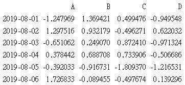
產生日期格式
pd.date_range()可以產生第一個參數開始的日期格式. 如下, 每列使用日期當索引, 欄位名為 ABCD四欄位
dates=pd.date_range("2019/08/01", periods=6)
df0=pd.DataFrame(np.random.randn(6,4), index=dates, columns=list('ABCD'))
print(df0)
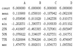
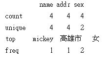
df.describe
describe可以求出每一欄位的數量, 平均值, 標準差…等資訊
df0.describe() 及 mem_df.describe()分別如下
其它功能
df.head(2) : 印前二個
df.tail(2) : 印後二個
df.transpose() : 轉置
df.sort_index(axis=1, ascending=True) :
axis=0: 對索引進行排序, axis=1 : 對欄位名稱排序
ascending : False 遞減
import pandas as pd
import numpy as np
dates=pd.period_range('2020/01/01', '2020/01/10')
rng=np.random.RandomState(1)
df=pd.DataFrame(rng.randn(len(dates),4), index=dates, columns=list('ABCD'))
print(df.sort_index(axis=0, ascending=False))
結果 :
                   A        B        C        D
2020-01-10 -1.117310 0.234416 1.659802 0.742044
2020-01-09 -0.687173 -0.845206 -0.671246 -0.012665
2020-01-08 -0.267888 0.530355 -0.691661 -0.396754
2020-01-07 0.900856 -0.683728 -0.122890 -0.935769
2020-01-06 -1.100619 1.144724 0.901591 0.502494
2020-01-05 -0.172428 -0.877858 0.042214 0.582815
2020-01-04 -0.322417 -0.384054 1.133769 -1.099891
2020-01-03 0.319039 -0.249370 1.462108 -2.060141
2020-01-02 0.865408 -2.301539 1.744812 -0.761207
2020-01-01 1.624345 -0.611756 -0.528172 -1.072969
import pandas as pd
import numpy as np
dates=pd.period_range('2020/01/01', '2020/01/10')
rng=np.random.RandomState(1)
df=pd.DataFrame(rng.randn(len(dates),4), index=dates, columns=list('ABCD'))
print(df.sort_index(axis=1, ascending=False))
結果 :
                   D         C         B        A
2020-01-01 -1.072969 -0.528172 -0.611756 1.624345
2020-01-02 -0.761207 1.744812 -2.301539 0.865408
2020-01-03 -2.060141 1.462108 -0.249370 0.319039
2020-01-04 -1.099891 1.133769 -0.384054 -0.322417
2020-01-05 0.582815 0.042214 -0.877858 -0.172428
2020-01-06 0.502494 0.901591 1.144724 -1.100619
2020-01-07 -0.935769 -0.122890 -0.683728 0.900856
2020-01-08 -0.396754 -0.691661 0.530355 -0.267888
2020-01-09 -0.012665 -0.671246 -0.845206 -0.687173
2020-01-10 0.742044 1.659802 0.234416 -1.117310
df.sort_values(by=’D’,ascending=False) : 使用D欄位遞減排序
df.index : 印出每列的索引
df.columns : 印出欄位名稱
df.values : 傳回每一列的list
df.shape : 傳回df的列數及行數
讀取儲存格資料
譊取行列的語法,採用 df.iloc[列, 行] ,列與行採用 “,” 隔開。多列或多行使用 “:” 隔開,如下語法
df.iloc[啟始列:結束列, 啟始行:結束行]
1. df.iloc[列, 行] : df.iloc[0,0]讀取第0列, 第0行的資料。請注意,索引編號由 0開始
2. df.iloc[列, [行, 行, 行]] : df.iloc[2,[0,1,2]] 讀取第2列, 0,1,2 行的資料. 使用values取出
3. df.iloc[列, :] : df.iloc[2,:] 讀取第2列所有行的資料. “:”代表所有行(或列). 使用values取出
3. df.iloc[:, 5] : df.iloc[:, 5] 讀取所有列第5列的資料. 使用values取出
import plotly_express as px
df = px.data.gapminder().query('year == 2007')
print('DataFrame 前 3 列資料')
for i in range(3):
    print(df.values[i])
print()

print('列印第0列第0,1,2欄')
row=df.iloc[0,[0,1,2]]
for c in row:
    print(f'{c} ', end='')
print('\n')

row=df.iloc[0,:]
print('第0列所有資料 :\n',row, '\n')
print('list :', list(row))
print('dict :', dict(row))
print('\n')

column=df.iloc[0:3,1]
print('第1行前3列的資料 :\n',column, '\n')
print(column)
print('list :', list(column))
print('dict :', dict(column))
print('\n')

結果:
DataFrame 前 3 列資料
['Afghanistan' 'Asia' 2007 43.828 31889923 974.5803384 'AFG' 4]
['Albania' 'Europe' 2007 76.423 3600523 5937.029525999998 'ALB' 8]
['Algeria' 'Africa' 2007 72.301 33333216 6223.367465 'DZA' 12]

列印第0列第0,1,2欄
Afghanistan Asia 2007

第0列所有資料 :
 country      Afghanistan
continent           Asia
year                2007
lifeExp           43.828
pop             31889923
gdpPercap     974.580338
iso_alpha            AFG
iso_num                4
Name: 11, dtype: object

list : ['Afghanistan', 'Asia', 2007, 43.828, 31889923, 974.5803384, 'AFG', 4]
dict : {'country': 'Afghanistan', 'continent': 'Asia', 'year': 2007, 'lifeExp': 43.828, 'pop': 31889923, 'gdpPercap': 974.5803384, 'iso_alpha': 'AFG', 'iso_num': 4}

第1行前3列的資料 :
11      Asia
23    Europe
35    Africa
Name: continent, dtype: object

11      Asia
23    Europe
35    Africa
Name: continent, dtype: object
list : ['Asia', 'Europe', 'Africa']
dict : {11: 'Asia', 23: 'Europe', 35: 'Africa'}
查詢功能
#設定搜尋條件
df=(df[df['country']=='Taiwan'])

#選取要列印的欄位
print(df[['country', 'year']])

#新增欄位
df['abb']=d['country'].apply(lambda x:x[:3])

#計算某欄位總合
print(df[df['year']==2007][['pop']].sum())

#計算多欄位的平均
print(df[df['year']==2007][['lifeExp', 'gdpPercap']].mean())
DataFrame視覺化
DataFrame 也可以視覺化製作圖表。但DataFrame使用matplotlib製作圖表,所以必需先
pip install matplotlib。
底下df[[list]] 中,list裏的欄位除了要有繪制圖表的資料外,也要包含要顯示在 x 軸及 y 軸的資料。list裏的資料如果是數字才會繪制,文字的部份就不會繪制。
x軸的標籤若要使用國別,可以在plot參數中加入 x=’country’
import plotly_express as px
import pylab as plt
df=px.data.gapminder().query("year==2007 and continent=='Asia'")
print(df.columns)
df[['country','pop']].plot(kind='bar', x='country')
plt.show()
讀取列 loc – 指定索引編號
底下的東西,本人覺的是 Pandas 在執行這個專案時未考慮到的多餘作法,只不過網路上還是有人用這些語法撰寫,所以還是記錄一下。
loc 可以指定索引編號讀取列,但傳入的索引 list 必需是索引編號存在的數字,比如經過 df.query(“year=2007”) 查詢後,索引編號只剩下 11, 23, 35, 47…..等1000多列。而0,1,2,….等編號都不在了。所以只能使用 df.loc[[11,23,35,47]],若使用 df.loc[[0,1,2,3,4,5]] 是錯誤的寫法。
另外也可以使用切片功能,比如 df.loc[0:50] 則列出索引編號 0~49 的列,不存在的索引則會去除。請注意 loc傳回的是 DataFrame格式。
import pandas as pd
import plotly_express as px
dis=pd.options.display
dis.max_columns=None
dis.max_rows=None
dis.width=None
dis.max_colwidth=None
df=px.data.gapminder()
df=df.query("year==2007")
print(df.loc[[11,23,35]])
print(df.loc[:50])
結果:
        country continent  year  lifeExp       pop    gdpPercap iso_alpha  iso_num
11  Afghanistan      Asia  2007   43.828  31889923   974.580338       AFG        4
23      Albania    Europe  2007   76.423   3600523  5937.029526       ALB        8
35      Algeria    Africa  2007   72.301  33333216  6223.367465       DZA       12
47       Angola    Africa  2007   42.731  12420476  4797.231267       AGO       24