什麼是強化學習

美國的心理學家 Skinner (史金納)，做一個叫 Skinner Box 的實驗裝置。把一隻飢餓的老鼠放到箱子裏，箱子中有一根桿子，按下桿子就會有食物掉出。實驗結果老鼠竟然學會了按下桿子，得到食物。

老鼠處於一種狀態(飢餓)。然後有二種選擇，也就是動作(壓桿子，或什麼事都不作)。最後產生結果，也就是回饋(有得吃或餓死)。飢餓狀態下會使按下桿子出現食物的機會大增，屬於正向回饋。發呆餓死為負向回饋，所以發呆的動作就會減少。這種藉由某個狀態強迫老鼠學習的方式，俗稱強迫學習，在此則稱為強化學習。

有養寵物的人也常使用這種強迫學習的方式，狗狗在家裏亂大小便，就把他關進籠子一小時，久了就會學乖了。狗狗也常會挑食，就讓他餓個二天，第三天就會乖乖的把飼料吃完。

現實世界中，狀態可能有很多種，動作也有很多種。為了知道在某種狀態下需採取什麼樣的動作，就需使用很有名的馬可夫決策。

馬可夫決策(Markov Decision Process, MDP)

Andrey Markov 是俄羅斯的數學家，主要研究在一連串相關事件所組成的系統中，會如何隨著時間變化。MDP定義如下的數學模型 :

狀態集合S : 有m種狀態，標示為 $(S=\{s_{0},s_{1},s_{2},….s_{m}\})$
動作函數A : A為可執行的動作集合
轉移模型$(P(s_{t+1}|s_{t}, a))$ : $(s_{t})$為當前狀態, $(s_{t+1})$為下一個狀態, a為時間為 t 時執行的動作
獎勵函數 R(s)
價值函數U(s)

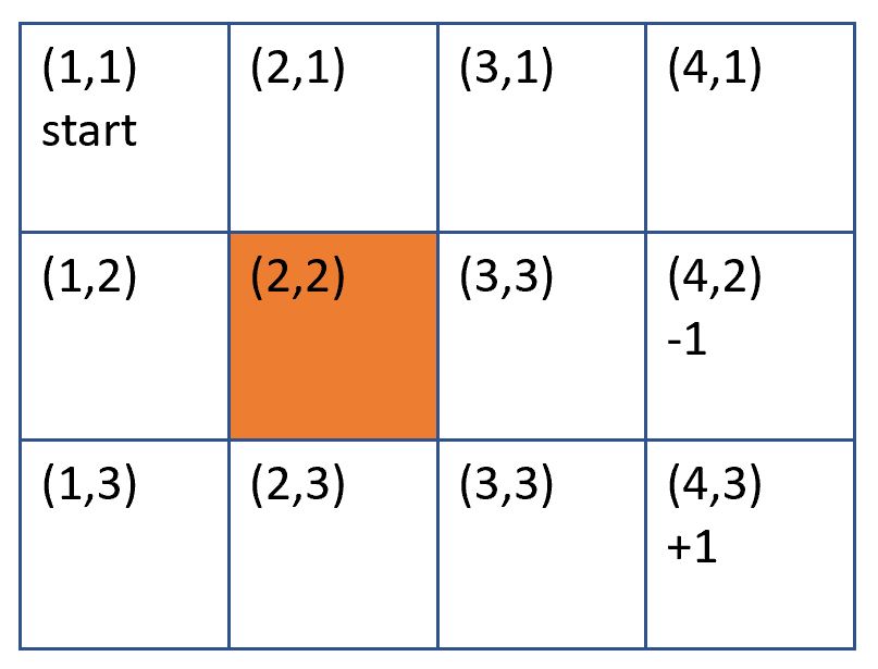
格子找路

上面四個集合或模型，實在是霧沙沙，所以用格子找路的例子說明。底下有 4*3 個格子，
1. 最初在 (1,1) 的格子
2. (2,2) 為一道牆，不能進入
3. 寶藏在(4, 3) 格，到達此格可加 1 分 (獎勵函數)
4. 陷井在 (4,2) 格，到達此格會減 1 分 (獎勵函數)
5. 每次移動 1 格，會消耗 0.04 分 (獎勵函數)

模型建立如下

狀態集合 : $(S=\{(x,y)|x\in \{1,2,3\},y\in \{1,2,3,4\} \})$
動作函數 : A={up, left, right, down}
轉移模型 : $(P(s_{t+1}|s_{t}, a))$ ，執行某動作後，轉移到下個狀態的機率
獎勵函數 : SCORE(s) = SCORE(x, y)，每個位置的得分(1, -1, 0, -0.04 )。

假設目前在 (1,3)，則 s=(1, 3)。往右走，則 a=right，此動作一定會成功，則 P((2,3)|(1, 3), right) = 100%。

獎勵分數為 $(SCORE(s)=\left\{\begin{matrix}
+1\;\;\;\;\;\;\;\;if\;\;\;s=(4, 3)\\
-1\;\;\;\;\;\;\;\;if\;\;\;s=(4, 2)\\
0\;\;\;\;\;\;\;\;\;if\;\;\;s=(2, 2)\\
-0.04\;\;\;\;\;\;\;\;other\;\;\;\;\;\;\;\;\;\;\;\;\;\;\;\;\;
\end{matrix}\right.)$

策略

策略 (policy) 定義為 $(\pi (s_{t}))$，指在狀態 $(s_{t})$ 時所推薦的動作。動作是 $(A(s_{t}))$ 集合，所以 $(\pi (s_{t}))$ 必然為 $(A(s_{t}))$ 其中之一。

最佳策略(best policy) 以 $(\pi^*(s_{t}))$ 表示，為狀態 $(s_{t})$ 時的最佳行動。

貝爾曼方程式

貝爾曼方程式是計算 s 狀態在 t 時間，往上下左右走到下一格時，取得那個一動作的最大值當作效用值。公式如下

$(U(s_{t})=R(s_{t})+ \gamma max E[P(s_{t+1}|s_{t}, a)U(s_{t+1})])$，

$(\gamma)$ 稱為折扣因子，愈接近 0 ，對效用愈不敏感。折扣因子愈接近 1 對效用愈敏感。

最佳路徑

貝爾曼公式看不懂也沒關係。請先看下面的程式，列出每格的回報值，最佳的走法是依較大的數值走就可得到最佳回報。

import numpy as np
def award(x, y):
    if (x==3 and y==2): return 1
    elif (x==3 and y==1):return -1
    elif (x==1 and y==1):return 0
    else:return -0.04
def exp(x, y):
    exp=[]
    if (x>0):exp.append((1*u[y][x-1]))
    if (x<3):exp.append(1*u[y][x+1])
    if (y>0):exp.append(1*u[y-1][x])
    if (y<2):exp.append(1*u[y+1][x])
    return exp
u=np.ones([3,4])
tmp=np.zeros([3,4])
epsilon=0.01
gamma=0.9
delta=100
#while delta >=epsilon *(1-gamma)/gamma:
while (u!=tmp).any():#二陣列只要有一個不相等, 就傳回True, 必需進行下一輪計算
    for y in range(3):
        for x in range(4):
            u[y][x]=tmp[y][x]
    delta=0
    for y in range(3):
        for x in range(4):
            if (x==3 and y==2) or (x==3 and y==1) or (x==1 and y==1):
                tmp[y][x]=award(x,y)
            else:
                e=exp(x, y)
                tmp[y][x]=award(x, y)+gamma * max(e)
            if abs(tmp[y][x]-u[y][x])>delta:
                delta=abs(tmp[y][x]-u[y][x])
print(u)
結果 : 
[[ 0.426686  0.51854   0.6206    0.51854 ]
 [ 0.51854   0.        0.734    -1.      ]
 [ 0.6206    0.734     0.86      1.      ]]

上述的max為策略，是指要獲得最大的回報數(走到 (4,3))。亦可以改為 min 獲得最小的回報(走到 (4,2))，如下結果所示

import numpy as np
def reward(x, y):
    if (x==3 and y==2): return 1
    elif (x==3 and y==1):return -1
    elif (x==1 and y==1):return 0
    else:return -0.04
def exp(x, y):
    exp=[]
    if (x>0):exp.append((1*u[y][x-1]))
    if (x<3):exp.append(1*u[y][x+1])
    if (y>0):exp.append(1*u[y-1][x])
    if (y<2):exp.append(1*u[y+1][x])
    return exp
u=np.ones([3,4])
tmp=np.zeros([3,4])
epsilon=0.01
gamma=0.9
delta=100
index=0
while (u!=tmp).any():
    index+=1
    for y in range(3):
        for x in range(4):
            u[y][x]=tmp[y][x]
    delta=0
    for y in range(3):
        for x in range(4):
            if (x==3 and y==2) or (x==3 and y==1) or (x==1 and y==1):
                tmp[y][x]=reward(x,y)
            else:
                e=exp(x, y)
                tmp[y][x]=reward(x, y)+gamma * min(e)
            if abs(tmp[y][x]-u[y][x])>delta:
                delta=abs(tmp[y][x]-u[y][x])
print(u)
print(index)
結果:
[[-0.79366  -0.8374   -0.886    -0.94    ]
 [-0.754294  0.       -0.94     -1.      ]
 [-0.79366  -0.8374   -0.886     1.      ]]

馬可夫性質給了一個定義 : 在狀態轉移過程中，下一個狀態只受到現在的狀態的影響，跟過去無關。馬可夫鏈可用 $(S_{n} = S \cdot T^n)$ 來計算第 n 次各種狀態的機率。

以寺廟中的筊杯作個例子，很多人可能不知道吧，聖杯 $(s_{0})$ 的機率是 0.5，笑杯 $(s_{1})$ 的機率是 0.25，無杯 $(s_{2})$ 的機率也是 0.25。如果第一次是聖杯，那第二次聖杯還是 0.5，笑杯0.25，無杯0.25。

底下的$(P(s_{n}|s_{n-1}))$ 表示由後面的 $(s_{n-1})$ 變成前面 $(s_{n})$ 的機率

狀態：一開始的狀態如果是聖杯，可以標示為　Ｓ＝[0.5 0.25 0.25]

轉移矩陣 : 可以標示為 $(T=\begin{bmatrix}
P(s_{0}|s_{0}) & P(s_{1}|s_{0}) & P(s_{2}|s_{0})\\
P(s_{0}|s_{1}) & P(s_{1}|s_{1}) & P(s_{2}|s_{1})\\
P(s_{0}|s_{2}) & P(s_{1}|s_{2}) & P(s_{2}|s_{2})
\end{bmatrix} = \begin{bmatrix}
0.5 & 0.25 & 0.25\\
0.5 & 0.25 & 0.25\\
0.5 & 0.25 & 0.25
\end{bmatrix})$

第一列的 $(\begin{bmatrix}
0.5 & 0.25 & 0.25
\end{bmatrix})$表示當前一次為聖杯時，下一次各種的機率
第二列的 $(\begin{bmatrix}
0.5 & 0.25 & 0.25
\end{bmatrix})$表示當前一次為笑杯時，下一次各種的機率
第三列的 $(\begin{bmatrix}
0.5 & 0.25 & 0.25
\end{bmatrix})$表示當前一次為沒杯時，下一次各種的機率

由下面的代碼來看，不論是第幾次筊杯，全都是聖杯0.5，笑杯0.25，沒杯0.25

import numpy as np
Matrix_trans = np.array([[0.5,0.25, 0.25],[0.5,0.25, 0.25],[0.5,0.25, 0.25]])
s0=np.array([0.5, 0.25, 0.25])
print('Initial state: \n', s0)
print('After 3 steps: \n', np.dot(s0, np.linalg.matrix_power(Matrix_trans, 3)))
print('After 5 steps: \n', np.dot(s0, np.linalg.matrix_power(Matrix_trans, 5)))
print('After 10 steps: \n', np.dot(s0, np.linalg.matrix_power(Matrix_trans, 10)))
print('After 15 steps: \n', np.dot(s0, np.linalg.matrix_power(Matrix_trans, 15)))
print('After 100 steps: \n', np.dot(s0, np.linalg.matrix_power(Matrix_trans, 100)))
print('After 200 steps: \n', np.dot(s0, np.linalg.matrix_power(Matrix_trans, 200)))
print('After 300 steps: \n', np.dot(s0, np.linalg.matrix_power(Matrix_trans, 300)))
Initial state: 
 [0.4  0.25 0.25]
After 3 steps: 
 [0.5  0.25 0.25]
After 5 steps: 
 [0.5  0.25 0.25]
After 10 steps: 
 [0.5  0.25 0.25]
After 15 steps: 
 [0.5  0.25 0.25]
After 100 steps: 
 [0.5  0.25 0.25]
After 200 steps: 
 [0.5  0.25 0.25]
After 300 steps: 
 [0.5  0.25 0.25]

好了，假設某個人卡到陰，先前是聖杯的話，下一次聖杯的機率為 0.5。先前若是笑杯的話，下一次沒杯的機率是0.6。先前若是沒杯，下一次沒杯的機率是0.7。

則轉移矩陣會變成 $(T= \begin{bmatrix}
0.5 & 0.25 & 0.25\\
0.2 & 0.2 & 0.6\\
0.15 & 0.15 & 0.7
\end{bmatrix})$

那麼再修改上面的代碼，變成如下，就會看到，在大約第20次時，就會收斂到
[0.24489796 0.18367347 0.57142857] 的機率。由這個機率就可以大膽的說，這個人真的是卡到陰了。

import numpy as np
Matrix_trans = np.array([[0.5,0.25, 0.25],[0.2,0.2, 0.6],[0.15,0.15, 0.7]])
s0=np.array([0.5, 0.25, 0.25])
print('Initial state: \n', s0)
print('After 3 steps: \n', np.dot(s0, np.linalg.matrix_power(Matrix_trans, 3)))
print('After 5 steps: \n', np.dot(s0, np.linalg.matrix_power(Matrix_trans, 5)))
print('After 10 steps: \n', np.dot(s0, np.linalg.matrix_power(Matrix_trans, 10)))
print('After 20 steps: \n', np.dot(s0, np.linalg.matrix_power(Matrix_trans, 20)))
print('After 100 steps: \n', np.dot(s0, np.linalg.matrix_power(Matrix_trans, 100)))
print('After 200 steps: \n', np.dot(s0, np.linalg.matrix_power(Matrix_trans, 200)))
print('After 300 steps: \n', np.dot(s0, np.linalg.matrix_power(Matrix_trans, 300)))
結果:
Initial state: 
 [0.5  0.25 0.25]
After 3 steps: 
 [0.25728125 0.18759375 0.555125  ]
After 5 steps: 
 [0.24655523 0.1841982  0.56924656]
After 10 steps: 
 [0.24490882 0.18367691 0.57141427]
After 20 steps: 
 [0.24489796 0.18367347 0.57142857]
After 100 steps: 
 [0.24489796 0.18367347 0.57142857]
After 200 steps: 
 [0.24489796 0.18367347 0.57142857]
After 300 steps: 
 [0.24489796 0.18367347 0.57142857]

todo

https://ithelp.ithome.com.tw/articles/10200744
https://ithelp.ithome.com.tw/articles/10215363

這篇寫的不錯
https://mofanpy.com/tutorials/machine-learning/reinforcement-learning/

馬可夫鍊

什麼是強化學習

馬可夫決策(Markov Decision Process, MDP)

格子找路

策略

貝爾曼方程式

最佳路徑

發佈留言