梯度下降是函數找極值的方法，如果應用在損失函數(迴歸線)，就是在找極小值的參數。比如
一階迴歸線 : $(y=ax+b)$，找尋 a, b 的值
二階迴歸線 : $(y=ax^2+bx+c)$，找尋 a, b, c 的值

本篇使用動畫說明每一步驟的變化。

使用 numpy 

假設 一元 6 階方程式為 $(y=0.001x^6-0.1x^5-0.68x^4+10000x^2+2)$ 

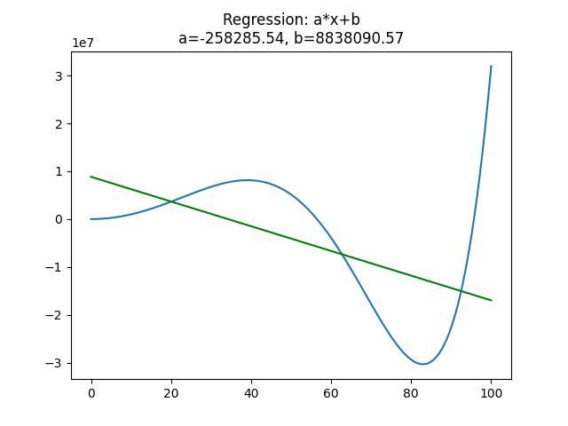
計算一階迴歸線

一階迴歸線的方程式為 $(y=ax+b)$，使用 numpy 計算出來的結果為
$(a*x + b=-258285.54*x + 8838090.57)$

import numpy as np
import pylab as plt
x=np.linspace(0,100, 10000000)
y=0.001*(x**6)-0.1*(x**5)-0.68*(x**4)+10000*(x**2)+2
plt.plot(x,y)

args=np.polyfit(x, y, 1)
f=np.poly1d(args)
plt.title(f'Regression: a*x+b\na={p[0]:.2f}, b={p[1]:.2f}')
plt.plot(x, f(x), 'g')
plt.show()

上述代碼執行後的結果如下

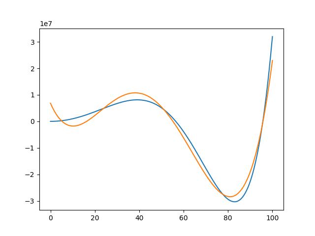
計算四階迴歸線

當 args=np.polyfit(x, y, 4) 作 4 階迴歸線時，迴歸線就愈接近實際值，列印的 args 值如下

[ 1.52290916e+01 -2.62626265e+03 1.31212114e+05 -1.92640644e+06
6.85425254e+06]

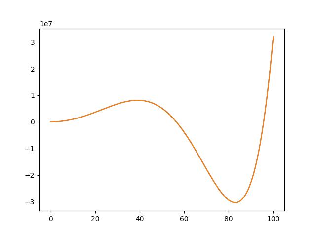
計算六階迴歸線

當 args=np.polyfit(x, y, 6) 作 6 階迴歸線時，迴歸線等於實際值。所得到的 args 值也幾乎等於方程式的每個參數。所以迴歸線就是使用每個點的值反推其原方程式。

[ 1.00000000e-03 -1.00000000e-01 -6.80000000e-01 -2.15229667e-11
1.00000000e+04 4.93033525e-10 2.00000004e+00]

計算八階迴歸線

args=np.polyfit(x, y, 8) 作 8 階迴歸線時，迴歸線也是等於實際值。但 args 多了二個 0 值。此時不但沒有提高精準度，反而耗時計算二個沒用的值，稱為 “過度擬合”。 

列印的參數如下

[ 3.51955078e-20 -1.32903585e-17 1.00000000e-03 -1.00000000e-01
-6.80000000e-01 -1.64237572e-10 1.00000000e+04 -6.90394067e-09
1.99999997e+00]

迴歸線或是PCA

損失函數的定義是 “實際值與預測值的差平方總合”。預測值如果是迴歸線產生出來的，那就是在計算迴歸線。但如果預測值是由 PCA 產生的，那就是計算 PCA 線。

實際與預測的最小值，不是只有這二種，還有其它的，以後還會有更多的理論。

一元一階梯度下降

依損失函數偏微分的說明，一階迴歸線的公式是 $(y=ax+b)$，
對 a 的偏微分是 $(=2\sum_{i=1}^{n}(\tilde{y_i}-y_i)x_i^1=2\sum_{i=1}^{n}(\tilde{y_i}-y_i)x_i)$
對 b 的偏微分是 $(=2\sum_{i=1}^{n}(\tilde{y_i}-y_i)x_i^0=2\sum_{i=1}^{n}(\tilde{y_i}-y_i))$

如果要儲存動畫，需先安裝套件

pip install celluloid

import pylab as plt
import numpy as np
from celluloid import Camera
fig=plt.figure(figsize=(9,6))
ax=plt.axes()
np.random.seed(1)
plt.rcParams['font.sans-serif'] = ['Microsoft JhengHei']

#解決UserWarning: Glyph 8722 (\N{MINUS SIGN}) missing from current font.
plt.rcParams['axes.unicode_minus']=False

n=20
x=np.linspace(-10,10 ,n)
y=0.5*x+3 + np.random.randint(-5,5, n)

#camera=Camera(fig)
epochs=200
a=0
b=0
lr=2.5e-3
# 一階迴歸線的公式 r = ax + b
r = a * x + b
diff=100000
pre_loss=100000
i=1
#for i in range(epochs):
while diff>0.001:
    ax.clear()
    ax.set_xlim(-15, 15)
    ax.set_ylim(-8, 15)
    ax.plot([-15,15], [0,0], c='k', linewidth=0.5)
    ax.plot([0,0], [-8,15], c='k', linewidth=0.5)
    ax.scatter(x, y, c='g')
    f=np.poly1d(np.polyfit(x, y, 1))
    ax.plot(x, f(x), c="b", linewidth=5)

    #開始梯度下降
    da = ((r - y) * (x ** 1)).sum()
    db = ((r - y)).sum()

    a = a - da * lr
    b = b - db * lr

    #計算損失函數的值
    r = a * x + b
    loss=np.square((y-r)).sum()
    diff=pre_loss-loss
    pre_loss=loss
    print(f'epochs : {i}, loss{loss}')
    ax.plot(x, a * x + b, c='r', linewidth=1)
    i += 1
    txt = f'逼近法迴歸函數 y={a:.7f}x+{b:.7f}'
    ax.text(-6, -7, txt, color='red')
    plt.pause(0.01)
#     camera.snap()
# animation=camera.animate()
# animation.save("loss_1.gif", writer='PillowWriter', fps=10)
plt.show()

Tensorflow版本

import pylab as plt
import numpy as np
import tensorflow as tf
from celluloid import Camera
fig=plt.figure(figsize=(9,6))
ax=plt.axes()
np.random.seed(1)
plt.rcParams['font.sans-serif'] = ['Microsoft JhengHei']

#解決UserWarning: Glyph 8722 (\N{MINUS SIGN}) missing from current font.
plt.rcParams['axes.unicode_minus']=False

n=20
x=np.linspace(-10,10 ,n)
y=0.5*x+3 + np.random.randint(-5,5, n)

#camera=Camera(fig)
a=tf.Variable(0.)#一定要用 tf.float32
b=tf.Variable(0.)
lr=9e-4
# 一階迴歸線的公式 r = ax + b
#r = a * x + b
diff=1
pre_loss=1_000_000_000

epoch=1
while diff>0.00001:
    dr=[]
    params=[a,b]
    for i in range(2):
        with tf.GradientTape() as tape:
            r = tf.reduce_sum(tf.pow(y - (a * x + b), 2))
        dr.append(tape.gradient(r, params[i]))
    ax.clear()
    ax.set_xlim(-15, 15)
    ax.set_ylim(-8, 15)
    ax.plot([-15,15], [0,0], c='k', linewidth=0.5)
    ax.plot([0,0], [-8,15], c='k', linewidth=0.5)
    ax.scatter(x, y, c='g')
    f = np.poly1d(np.polyfit(x, y, 1))
    ax.plot(x, f(x), c="b", linewidth=5)

    a = tf.Variable(a- dr[0] * lr)
    b = tf.Variable(b- dr[1] * lr)
    #計算損失的值
    loss = tf.reduce_sum(tf.pow(y - r, 2)).numpy()/1e6
    diff=pre_loss-loss
    pre_loss=loss
    print(f'epochs : {epoch}, loss : {loss}, diff:{diff}')
    epoch += 1
    ax.plot(x, a * x + b, c='r', linewidth=1)

    txt = f'逼近法迴歸函數 y={a.numpy():.7f}x+{b.numpy():.7f}'
    ax.text(-6, -7, txt, color='red')
    plt.pause(0.01)
#     camera.snap()
# animation=camera.animate()
# animation.save("loss_1.gif", writer='PillowWriter', fps=10)
plt.show()

一元四階梯度下降

依損失函數偏微分的說明，四階迴歸線的公式是 $(y=ax^4+bx^3+cx^2+dx+e)$，
對 a 的偏微分是 $(=2\sum_{i=1}^{n}(\tilde{y_i}-y_i)x_i^4)$
對 b 的偏微分是 $(=2\sum_{i=1}^{n}(\tilde{y_i}-y_i)x_i^3)$
對 c 的偏微分是 $(=2\sum_{i=1}^{n}(\tilde{y_i}-y_i)x_i^2)$
對 d 的偏微分是 $(=2\sum_{i=1}^{n}(\tilde{y_i}-y_i)x_i^3)$
對 e 的偏微分是 $(=2\sum_{i=1}^{n}(\tilde{y_i}-y_i)x_i^0)$
梯度下降逼近的代碼如下。

import pylab as plt
import numpy as np
from celluloid import Camera
fig=plt.figure(figsize=(9,6))
ax=plt.axes()
np.random.seed(1)
plt.rcParams['font.sans-serif'] = ['Microsoft JhengHei']

#解決UserWarning: Glyph 8722 (\N{MINUS SIGN}) missing from current font.
plt.rcParams['axes.unicode_minus']=False

n=20
x=np.linspace(-10,10 ,n)
y=0.5*x+3 + np.random.randint(-5,5, n)

#camera=Camera(fig)
epochs=500
a=0
b=0
c=0
d=0
e=0
lr=2.5e-3
r = a * (x ** 4) + b * (x ** 3) + c * (x ** 2) + d * x + e
diff=100000
pre_loss=100000
#for i in range(epochs):
i=1
while diff>0.0001:
    ax.clear()
    ax.set_xlim(-15, 15)
    ax.set_ylim(-8, 15)
    ax.plot([-15,15], [0,0], c='k', linewidth=0.5)
    ax.plot([0,0], [-8,15], c='k', linewidth=0.5)
    ax.scatter(x, y, c='g')
    f=np.poly1d(np.polyfit(x, y, 4))
    ax.plot(x, f(x), c="b", linewidth=5)

    #開始逼近
    da = ((r - y) * (x ** 4)).sum()
    db = ((r - y) * (x ** 3)).sum()
    dc = ((r - y) * (x ** 2)).sum()
    dd = ((r - y) * x).sum()
    de = ((r - y)).sum()

    a = a - da * lr / 1e6
    b = b - db * lr / 1e4
    c = c - dc * lr / 1e3
    d = d - dd * lr / 1e1
    e = e - de * lr / 1e0

    r = a * (x ** 4) + b * (x ** 3)+ c * (x ** 2) +d * x + e
    ax.plot(x, r, c='r', linewidth=1)

    #計算損失函數的值
    loss=np.square(r - y).sum()
    diff=pre_loss-loss
    pre_loss=loss
    print(f'epochs : {i} : loss : {loss}')
    i+=1
    txt = f'逼近法迴歸函數 y={a:.7f}x^4+{b:.7f}x^3+{c:.7f}x^2+{d:.7f}x+{e:.7f}'
    ax.text(-12, -7, txt, color='red')
    #camera.snap()
    plt.pause(0.01)

# animation = camera.animate()
# animation.save('reg_ani.gif', writer='PillowWriter', fps=10)
plt.show()

結果 : 
.....................
epochs : 969 : loss : 119.32315850329866
epochs : 970 : loss : 119.3230572088199
epochs : 971 : loss : 119.32295658324597
epochs : 972 : loss : 119.32285662215968

Tensorflow 版

import pylab as plt
import numpy as np
import tensorflow as tf
from celluloid import Camera
fig=plt.figure(figsize=(9,6))
ax=plt.axes()
np.random.seed(1)
plt.rcParams['font.sans-serif'] = ['Microsoft JhengHei']

#解決UserWarning: Glyph 8722 (\N{MINUS SIGN}) missing from current font.
plt.rcParams['axes.unicode_minus']=False

n=20
x=np.linspace(-10,10 ,n)
y=0.5*x+3 + np.random.randint(-5,5, n)

#camera=Camera(fig)
a=tf.Variable(0.)#一定要用 tf.float32
b=tf.Variable(0.)
c=tf.Variable(0.)
d=tf.Variable(0.)
e=tf.Variable(0.)
lr=9e-4
# 一階迴歸線的公式 r = ax + b
#r = a * x**x + b * x**3 +c *x**2 +d * x +e
diff=1
pre_loss=1e9
epoch=1
while diff>1e-6:
    dr=[]
    params=[a,b,c,d,e]
    for i in range(5):
        with tf.GradientTape() as tape:
            r = tf.reduce_sum(tf.pow(y - ( a * x**4 + b * x**3 +c * x**2 +d * x +e), 2))
        dr.append(tape.gradient(r, params[i]))
    ax.clear()
    ax.set_xlim(-15, 15)
    ax.set_ylim(-8, 15)
    ax.plot([-15,15], [0,0], c='k', linewidth=0.5)
    ax.plot([0,0], [-8,15], c='k', linewidth=0.5)
    ax.scatter(x, y, c='g')
    f = np.poly1d(np.polyfit(x, y, 4))
    ax.plot(x, f(x), c="b", linewidth=5)

    a = tf.Variable(a - dr[0] * lr/1e6)
    b = tf.Variable(b - dr[1] * lr/1e5)
    c = tf.Variable(c - dr[2] * lr/1e3)
    d = tf.Variable(d - dr[3] * lr/1e1)
    e = tf.Variable(e - dr[4] * lr)
    #計算損失的值
    loss = tf.reduce_sum(tf.pow(y - r, 2)).numpy()/1e6
    diff=pre_loss-loss
    pre_loss=loss
    print(f'epochs : {epoch}, loss : {loss}, diff:{diff}')
    epoch += 1
    ax.plot(x,  a * x**4 + b * x**3 +c *x**2 +d * x +e, c='r', linewidth=1)

    txt = f'逼近法迴歸函數 y={a.numpy():.7f}x^4+{b.numpy():.7f}x^3+{c.numpy():.7f}x^2+{d.numpy():.7f}x+{e.numpy():.7f}'
    ax.text(-12, -7, txt, color='red')
    plt.pause(0.01)
#     camera.snap()
# animation=camera.animate()
# animation.save("loss_1.gif", writer='PillowWriter', fps=10)
plt.show()

新版程式

import pylab as plt
import numpy as np
import tensorflow as tf
fig=plt.figure(figsize=(9,6))
ax=plt.axes()
np.random.seed(1)
#plt.rcParams['font.sans-serif'] = ['Microsoft JhengHei']

#解決UserWarning: Glyph 8722 (\N{MINUS SIGN}) missing from current font.
#plt.rcParams['axes.unicode_minus']=False

n=20
x=np.linspace(-10,10 ,n)
y=0.5*x+3 + np.random.randint(-5,5, n)
a=tf.Variable(0.)
b=tf.Variable(0.)
c=tf.Variable(0.)
d=tf.Variable(0.)
e=tf.Variable(0.)
lr=9e-4
diff=1
pre_loss=1e9
p = ["a", "b", "c", "d", "e"]
l=len(p)
str_f=""
for i in range(l):
    str_f+=f'{p[i]}*x**{l-1-i}+'
str_f=str_f[:-1]
str_loss=f"tf.reduce_sum(tf.square(y-({str_f})))"

print(str_loss)
epoch=0
while diff>1e-6:
    ax.clear()
    ax.set_xlim(-15, 15)
    ax.set_ylim(-8, 15)
    ax.plot([-15,15], [0,0], c='k', linewidth=0.5)
    ax.plot([0,0], [-8,15], c='k', linewidth=0.5)
    ax.scatter(x, y, c='g')
    f = np.poly1d(np.polyfit(x, y, 4))
    ax.plot(x, f(x), c="b", linewidth=5)
    dr=[]
    params=[a,b,c,d,e]
    for i in range(len(params)):
        with tf.GradientTape() as tape:
            r=eval(str_loss)
        dr.append(tape.gradient(r, params[i]))
    a = tf.Variable(a - dr[0] * lr/1e6)
    b = tf.Variable(b - dr[1] * lr/1e5)
    c = tf.Variable(c - dr[2] * lr/1e3)
    d = tf.Variable(d - dr[3] * lr/1e1)
    e = tf.Variable(e - dr[4] * lr)
    #計算損失的值
    loss = tf.reduce_sum(tf.pow(y - r, 2)).numpy()/1e6
    diff=pre_loss-loss
    pre_loss=loss
    print(f'epochs : {epoch}, loss : {loss}, diff:{diff}')
    epoch += 1
    ax.plot(x,  eval(str_f), c='r', linewidth=1)
    print(f'epoch:{epoch}')

    plt.pause(0.1)
plt.show()

二元損失函數

二元方程式 $(z=\frac{z=0.006x^6-0.005y^6+0.5x^5-0.1y^5+0.005x^4+0.003y^4}{10000000})$

二元一階迴歸(面)線為 $(y=ax+by+c)$，

下圖的迴歸面， a = 0.9，b =1.8，c = 200，怎麼算出來的? 那是本人瞎掰的，最終還是要使用梯度下降法來求。

import plotly
import plotly.graph_objs as go
import numpy as np
import pandas as pd
display=pd.options.display
display.max_columns=None
display.max_rows=None
display.width=None
display.max_colwidth=None
n=100
z=np.zeros([n, n])
for x in range(n):
    for y in range(n):
        z[x, y] = (0.0006 * x ** 6 - 0.005 * y ** 6 + 0.5 * x ** 5 - 0.1 * y ** 5 + 0.005 * x ** 4 + 0.003 * y ** 4) / 10000000
#z 必需是二維的陣列或 list
trace1=go.Surface(z=z)

a=0.9
b=1.8
c=-200
for x in range(n):
    for y in range(n):
        z[x, y] = a*x+b*y+c
trace2=go.Surface(z=z, coloraxis='coloraxis')
data=[trace1, trace2]
layout=go.Layout(title=f'Regression : a*x+b*y+c', autosize=True,margin=dict(l=0, r=0, b=0, t=40))
fig=go.Figure(data=data, layout=layout)
fig.show()

地型圖

地型圖也可以用 2 元 n 階方程式來表示，但方程式非常猙獰且複雜，所以只好使用這些點產生一個回歸面，再由 (x, y) 算出這個迴歸面的值來預估。展示圖片的代碼如下

import plotly
import plotly.graph_objs as go
import numpy as np
import pandas as pd

df = pd.read_csv(
    'https://raw.githubusercontent.com/plotly/datasets/master/api_docs/mt_bruno_elevation.csv',
    dtype='float')

trace1=go.Surface(z=df.values)
n=df.shape[0]
z=np.zeros([n, n])
a=0.9
b=1.8
c=50
for x in range(n):
    for y in range(n):
        z[x, y] = a*x+b*y+c
trace2=go.Surface(z=z, coloraxis='coloraxis1')
data=[trace1, trace2]
layout=go.Layout(title=f'Regression : a*x+b*y+c', autosize=True,margin=dict(l=0, r=0, b=0, t=40))
fig=go.Figure(data=data, layout=layout)
fig.show()

多元迴歸線

其實並沒有迴歸面這個名詞，我們統一稱為 “多元迴歸線”。多元迴歸線的公式為

$(f(x_1, x_2, x_3, x_4…)=ax_1+bx_2+cx_3+dx_4+……)$

todo

後續工作

1. a, b, c,…. 的初始值該如何定才能加速收斂。
2. 如何加速梯度下降。
3. 學習率該如何定。
4. 要訓練幾次(epochs)。