tensorflow 有些常用的函數，需要仔細的背起來

tf.random.normal

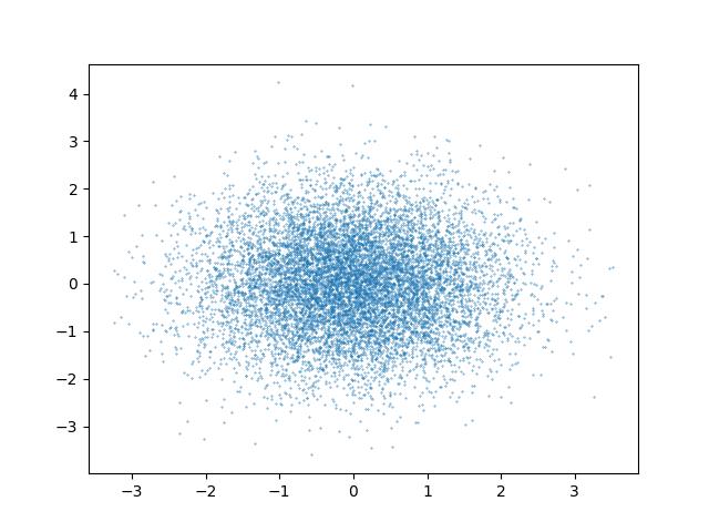
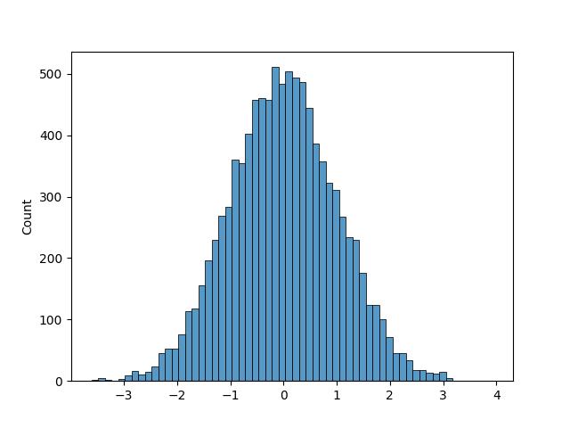
標準常態分佈亂數會在大部份集中於0左右的小數亂數。其實np.random.normal()也可以產生此功能。

import os
os.environ['TF_CPP_MIN_LOG_LEVEL']='2'
import tensorflow as tf
import pylab as plt
import seaborn as sns
batch=10000
x=tf.random.normal([batch])
y=tf.random.normal([batch])
#plt.scatter(x, y, s=0.1)
sns.histplot(x)
plt.savefig("tf_normal_histplot.jpg")
plt.show()

plt點散圖如下

海生圖如下

tf.random.uniform

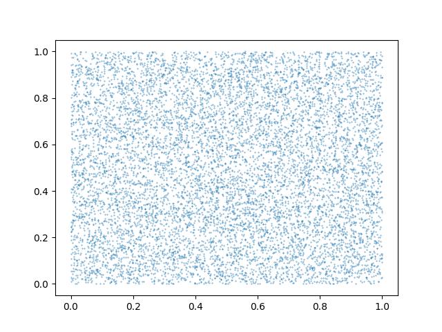
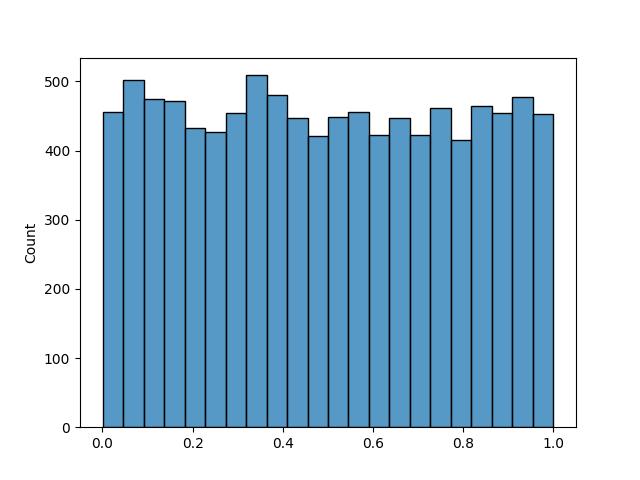
在陣列這篇的說明，有提到 tf.random.uniform是產生均勻分佈陣列的函數，參數只需傳入要產生亂數的數量即可。另外 tf.random.unifomr 還可以下達 minval 及 maxval 設定最小值及最大值，但不包含最大值。

底下代碼可以產生均勻分佈亂數

import os
os.environ['TF_CPP_MIN_LOG_LEVEL']='2'
import numpy as np
import tensorflow as tf
import pylab as plt
import seaborn as sns
batch=10000
x=tf.random.uniform([batch])
y=tf.random.uniform([batch])
plt.scatter(x, y, s=0.1)
#sns.histplot(y)
print(y.numpy())
plt.savefig("tf_uniform_scatter.jpg")
plt.show()

plt點散圖如下

海生圖分佈狀態如下

產生均勻分佈亂數，其實也可以用 np. random.uniform(0, 1, batch)。這二個有什麼不同呢? 當產生的數量多達1億個的時候，這二個所花費的時間差不多是在 0.4 秒左右，但如果產生的數量大於 1 億，numpy 的效能就會遠遠落後 tf 很多。

import os
import time
os.environ['TF_CPP_MIN_LOG_LEVEL'] = '2'
import tensorflow as tf
import numpy as np
batch=500_000_000
t1=time.time()
a=tf.random.uniform([batch])
t2=time.time()
print(f'tf花費 : {t2-t1}秒')

t1=time.time()
b=np.random.uniform(0, 1, batch)
t2=time.time()
print(f'np花費 : {t2-t1}秒')
結果 : 
tf花費 : 0.4383711814880371秒
np花費 : 2.5611190795898438秒

tf.sqrt

sqrt 為求取平方的函數，只能用於小數型態。如果是整數型態，會發生例外錯誤。

另外如果傳入的型態是陣列的話，就會將陣列中的每一個元素進行運算。

import os
os.environ['TF_CPP_MIN_LOG_LEVEL'] = '2'
import tensorflow as tf

#tf.sqrt只能用在小數型態
a=tf.constant(10.)
print(tf.sqrt(a))

#底下為整數型態，無法使用 sqrt
#b=tf.constant(10)
#print(tf.sqrt(b))
c=tf.constant([1., 2., 3.])
print(tf.sqrt(c))
結果 : 
tf.Tensor(3.1622777, shape=(), dtype=float32)
tf.Tensor([1.        1.4142135 1.7320508], shape=(3,), dtype=float32)

numpy 也有 np.sqrt 的方法，底下對 1 億個數字進行進算，可見 tf.sqrt 效能遠遠比 numpy 好很多

import os
os.environ['TF_CPP_MIN_LOG_LEVEL'] = '2'
import tensorflow as tf
import numpy as np
import time
batch=100_000_000
t1=time.time()
a=tf.random.uniform([batch])
t2=time.time()
print(f'tf產生亂數花費 : {t2-t1}秒')

t1=time.time()
b=np.random.uniform(0, 1, batch)
t2=time.time()
print(f'np產生亂數花費 : {t2-t1}秒')


t1=time.time()
a=tf.sqrt(a)
t2=time.time()
print(f'tf計算平方花費 : {t2-t1}秒')

t1=time.time()
b=np.sqrt(b)
t2=time.time()
print(f'np計算平方花費 : {t2-t1}秒')
結果:
tf產生亂數花費 : 0.44187140464782715秒
np產生亂數花費 : 0.5215818881988525秒
tf計算平方花費 : 0.0009970664978027344秒
np計算平方花費 : 0.14860248565673828秒

tf.square

tf.square為求取平方值，適用於整數及小數。同樣如果是陣列，也會足一將每個元素的平方計算一遍。

import os
os.environ['TF_CPP_MIN_LOG_LEVEL'] = '2'
import tensorflow as tf

a=tf.constant(10.)
print(tf.square(a))

b=tf.constant(10)
print(tf.square(b))
結果 :
tf.Tensor(100.0, shape=(), dtype=float32)
tf.Tensor(100, shape=(), dtype=int32)

tf.where

where後面的參數為條件，此法可將陣列中符合條件的索引值集合成一個新的 n*1 的 Tensor 陣列。
如果要取出符合的值，需使用 value = tf.gather(x, idx)。
最後若要得知符合的數量，使用 value.shape[0]。

import os
os.environ['TF_CPP_MIN_LOG_LEVEL'] = '2'
import tensorflow as tf
batch=10
x=tf.random.uniform([batch])
print(f'原始資料 : {x}')
idx=tf.where(x<=0.5)
print(f'符合的索引 :\n{idx}')
value=tf.gather(x, idx)
print(f'符合的值 : {value}')
print(f'符合的數量 : {value.shape[0]}')
原始資料 : [0.5912652  0.97370183 0.21289659 0.52576315 0.13146174 0.76325166
 0.10665309 0.54943335 0.59710836 0.76287985]
符合的索引 :
[[2]
 [4]
 [6]]
符合的值 : [[0.21289659]
 [0.13146174]
 [0.10665309]]
符合的數量 : 3

導數

導數就是微分，微分就是導數。比如$(f(x)=x^{2})$，經過一次微分後，結果為$(f'(x)=2x)$，所以當x=3時，$(y=f'(x)=6)$

with tf.GradientTape() as prototype 的區塊中，就是在宣告函數的原型。然後再使用y_grad=prototype.gradient(x, y)就可以求取y對x的導數。

import os
os.environ['TF_CPP_MIN_LOG_LEVEL']='2'
import tensorflow as tf
cpus=tf.config.experimental.list_physical_devices(device_type='CPU')
tf.config.set_visible_devices(devices=cpus)
x = tf.Variable(3.)
with tf.GradientTape() as prototype:#宣告原型函數
    y = tf.pow(x, 2)
y_grad = prototype.gradient(y, x)# 計算y關於x的導數
print('y=x^2, x=3, y=',y)
print('一次微分後，y導數=', y_grad)
結果 :
y=x^2, x=3, y= tf.Tensor(9.0, shape=(), dtype=float32)
一次微分後，y導數= tf.Tensor(6.0, shape=(), dtype=float32)

損失函數偏導數

$(x=\begin{bmatrix}1 & 2\\ 3 & 4 \end{bmatrix})$ , $(y=\begin{bmatrix}1\\2\end{bmatrix})$ , $(w=\begin{bmatrix}1\\2\end{bmatrix})$ , $(b=1)$

假設 y=xw + b ，則底下為其損失函數

$(L(w, b)=\sum (xw+b-y )^{2})$

import tensorflow as tf
X = tf.constant([[1., 2.], [3., 4.]])
y = tf.constant([[1.], [2.]])
w = tf.Variable(initial_value=[[1.], [2.]])
b = tf.Variable(initial_value=1.)
with tf.GradientTape() as tape:
    L = tf.reduce_sum(tf.square(tf.matmul(X, w) + b - y))
w_grad, b_grad = tape.gradient(L, [w, b])        # 計算L(w, b)關於w, b的偏導數
print(L)
print(w_grad)
print(b_grad)
結果:
tf.Tensor(125.0, shape=(), dtype=float32)
tf.Tensor(
[[ 70.]
[100.]], shape=(2, 1), dtype=float32)
tf.Tensor(30.0, shape=(), dtype=float32)

todo

tf2 常用函數