
機器學習與深度學習
深度學習是屬於機器學習其中一個分支,深度學習不需要輸入特徵,會自已去找特徵。
不過此房價預測範例必需輸入特徵,所以不屬於深度學習範圍。那為何把此專案例入深度學習呢??
在此必需承認一件事,前面的 AI人工智慧 章節混合了 “非深度學習” 及 “深度學習” 的課程。如今新增了深度學習的課程,所以必需強加區隔。在以往的 AI人工智慧 並未介紹如何由特徵進行分析,所以由此開始介紹。
波士頓房價預測
盡管我們 (應該說是本人) 對房價不是那麼的關心 (就買不起咩),更何況這是波士頓的房價狀況。但這一道題目是許多機器學習者的起手式,裏面的資料完整且多人討論,所以只能由此開始。其實還是有點小小的願望啦,希望能預測到準確的房價,在最低點時出手,賺那麼一小筆。
房價預測案例源自於 Kaggle網站,Kaggle 是一個數據建模和數據分析競賽平台,開發者都可以在上面發佈數據。由於研究人員不可能在一開始就知道要用什麼方法來解決特定的問題是最有效的,所以Kaggle就透過眾人的經驗來解決此一問題。Kaggle於2017/03/08 已被 Google 正式收購。
資料下載
請到 kaggle 官網下載相關資料。請點選 Data,然後往下拉,就會看到 train.csv及test.csv二個檔。下載前必需先登入。若不想登入,請由本站下載。
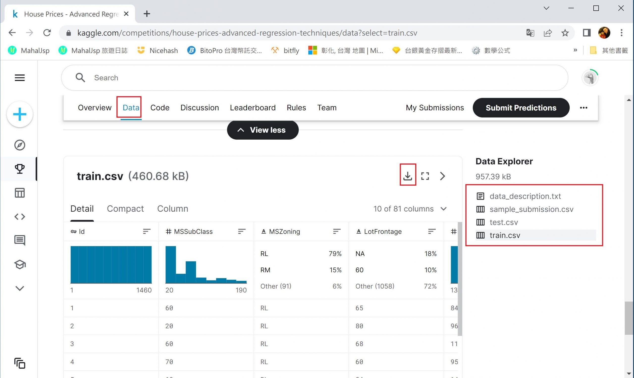
上面的 train.csv 共有1641筆資料,每筆料共有81個特徵。
安裝套件
pip install xgboost lightgbm mlxtend
步驟流程
此例需連行EDA,特徵工程,模型訓練,模型融合等四項工作
EDA(Explorator Data Analysis)
資料分析探索 (Explorator Data Analysis) 是讓我們對收集到的資料有充分的了解。包含了
房價分佈 : 每個房價的分佈圖
相關特徵 : 那些事情 (特徵) 對房價的影響特別力害,
無關特徵 : 那些事情 (特徵) 對房價沒啥影響。
相關欄位(特徵)
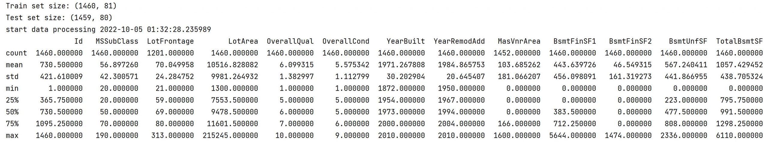
train.csv共有1460筆資料,每筆資料有81個欄位。在資料庫裏,我們稱欄位,但在機器學習裏,就是我們所說的特徵。底下的代碼中,train為 DataFrame格式,所以可以使用 describe來計算每個欄位的數量、平均值、標準差…
請使用 Pycharm開啟新專案,然後將train.csv及 test.csv copy 到專案下的 kaggle目錄。開始執行此程式時,請先安裝如下套件
pip install seaborn matplotlib numpy xlrd openpyxl
然後開啟 模型訓練.py檔
import pandas as pd
from datetime import datetime
display=pd.options.display
display.max_columns=None
display.max_rows=None
display.width=None
display.max_colwidth=None
train = pd.read_csv('kaggle/train.csv')
test = pd.read_csv('kaggle/test.csv')
print("Train set size:", train.shape)
print("Test set size:", test.shape)
print('start data processing', datetime.now(), )
print(train.describe())
#print(train['SalePrice'].describe())
房價分析
房價分析如下代碼
#查看房價的偏移及峰值
import seaborn as sns
import pylab as plt
sns.distplot(train['SalePrice'])
plt.show()
結果如下
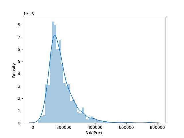
房價的偏移值稍往左邊,且峰值較徒,需使用 log進行修正,如下。
修正skewness 及 kurtosis
skewness 為偏移值, kurtosis 為峰值。上述的圖型中,房價的 skew 及 kurt 都出 1的值,所以使用 log 值修正在1 之內,如下
#修正過大的偏移及峰值
import numpy as np
print("修正前 Skewness: %f" % train['SalePrice'].skew())
print("修正前 Kurtosis: %f" % train['SalePrice'].kurt())

#log變換可以解決此問題,而且損失函數也是 log-rmse,後面會對SalePrice作log--transformation
train["SalePrice"] = np.log1p(train["SalePrice"])
print("修正後 Skewness: %f" % train['SalePrice'].skew())
print("修正後 Kurtosis: %f" % train['SalePrice'].kurt())
結果:
修正前 Skewness: 1.882876
修正前 Kurtosis: 6.536282
修正後 Skewness: 0.121347
修正後 Kurtosis: 0.809519
請注意喔,若不修正在 1 之內,後續的分析,會不準確
特徵關連 – 皮爾森積差
https://ithelp.ithome.com.tw/articles/10205038
Pearson (皮爾森) 積差相關係數其實就是 pandas Dataframe 的 corr 方法。
Pearson 係數是在測量各個特徵之間的線性關係。係數值在 -1 和 +1 之間變化,0表示它們之間沒有相關性,接近 -1 或 +1 代表有極強的線性關係。pandas .corr 計算每一個特徵和其餘所有特徵的皮爾遜積差相關係數。皮爾森系數只是一堆數字,人類是無法理解的,所以總是使用熱度圖來視覺化皮爾森積差相關係數:
熱度圖使用了顏色來做關聯性的區分,熱度圖中顏色越極端 (接近全白、全黑) 的格子代表關聯性越強的表徵。熱度圖中有一條對角的全白線,此現象應該忽略,因為它是代表表徵與他自己本身的關聯性自然為1。
import pandas as pd
import seaborn as sns
import pylab as plt
import numpy as np
train = pd.read_csv('kaggle/train.csv')
test = pd.read_csv('kaggle/test.csv')
corrmat = train.corr()
#取 前 10名
k = 10
cols = corrmat.nlargest(k, 'SalePrice')['SalePrice'].index
cm = np.corrcoef(train[cols].values.T)
sns.set(font_scale=1.25)
hm = sns.heatmap(cm,
                 cbar=True,
                 annot=True,
                 square=True,
                 fmt='.2f',
                 annot_kws={'size': 10},
                 yticklabels=cols.values,
                 xticklabels=cols.values)
plt.show()
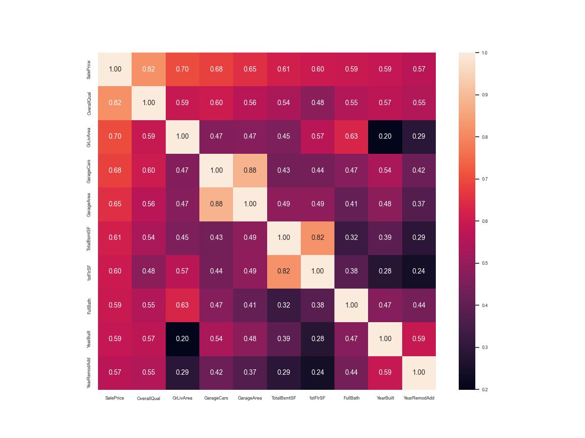
先解說一下上述特徵的縮寫,
SalePrice是房價,
OverallQual 是方房屋材料裝潢,
GrLiveArea地面居住面積,
GarageCars車庫容積,
TotalBsmtSF地下室面積。
房價跟上面那幾個有很強的關聯性。
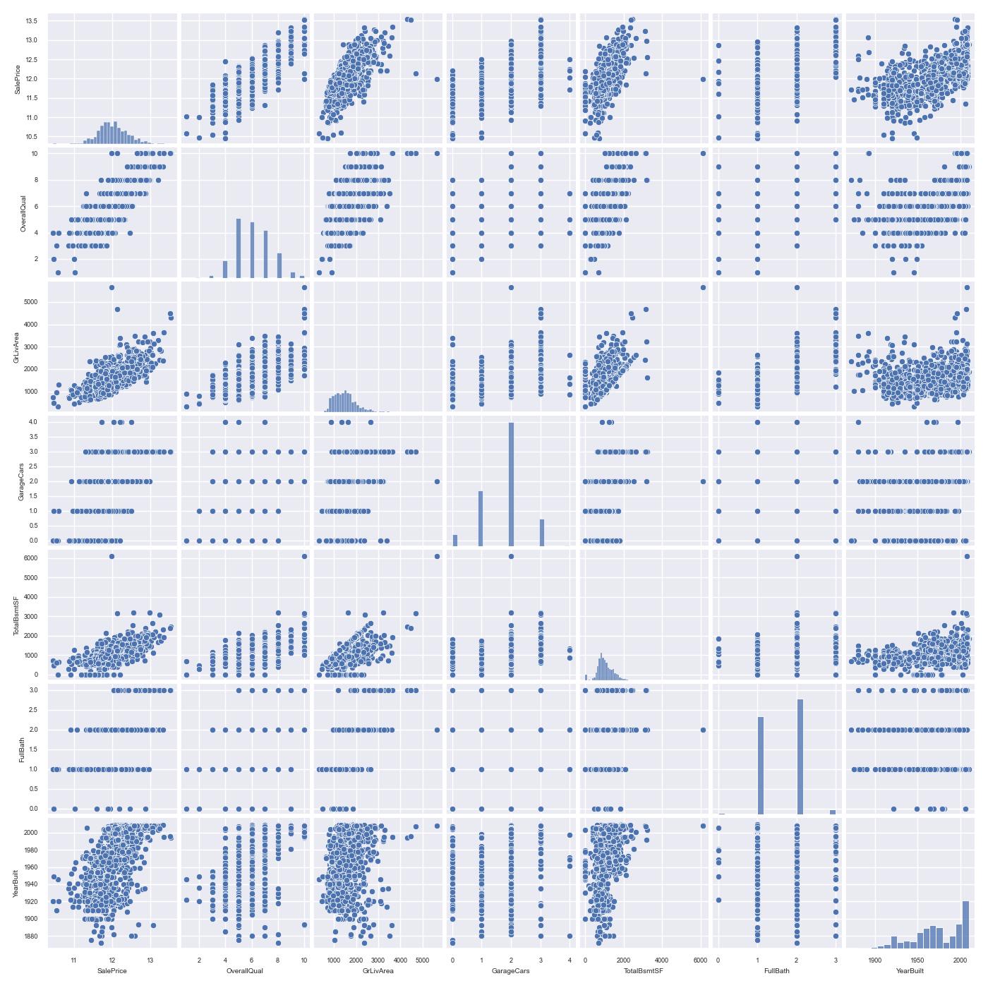
成對關係圖
上面的熱度圖可以看出幾點
- OverallQual、GrLivArea、TotalBsmtSF 與 SalePrice 有很強的關連性。
- GarageCars 和 GarageArea 也是強關連變量. 但車量數由車庫面積決定,它們就像雙胞胎。所以只需一個變數即可,我們選擇GarageCars,因為其實0.68比較高。
- TotalBsmtSF 和 1stFloor 與上述一樣選擇 TotalBsmtS 。
- FullBath 也是強關連。
- YearBuilt 和 SalePrice 也是強關連。
底下的pairplot可以畫出成對的海生圖。其對角皆為直方圖
sns.set(font_scale=0.6)
cols = ['SalePrice', 'OverallQual', 'GrLivArea', 'GarageCars', 'TotalBsmtSF', 'FullBath', 'YearBuilt']
sns.pairplot(train[cols], size = 1.5)
刪除離群樣本
在中等高維數據集中檢測離群樣本的方法,可以使用scikit-learn 區域性異常因子檢測函數 LocalOutlierFactor。LOF的演算法將於下一篇的 Local Outlier Factor 進行說明。
底下的程式刪除離群樣本後,會印出(1453, 81),也就是說,只剩下1453筆資料沒有離群
#刪除離群樣本
from sklearn.neighbors import LocalOutlierFactor
def detect_outliers(x, y, top=5, plot=True):
    lof = LocalOutlierFactor(n_neighbors=40, contamination=0.1)
    x_ =np.array(x).reshape(-1,1)
    preds = lof.fit_predict(x_)
    lof_scr = lof.negative_outlier_factor_
    out_idx = pd.Series(lof_scr).sort_values()[:top].index
    if plot:
        f, ax = plt.subplots(figsize=(9, 6))
        plt.scatter(x=x, y=y, c=np.exp(lof_scr), cmap='RdBu')
    return out_idx
outliers = [30, 88, 462, 523, 632, 1298, 1324]
all_outliers=[]
numeric_features = train.dtypes[train.dtypes != 'object'].index
for feature in numeric_features:
    try:
        outs = detect_outliers(train[feature], train['SalePrice'],top=5, plot=False)
    except Exception as e:
        continue
    all_outliers.extend(outs)
print(all_outliers)
#刪除離群資料
train = train.drop(train.index[outliers])
print(train.shape)
合併train及 test資料
為什麼要合併呢,只是為了下面的特徵工程而以。因為 test並沒有 SalePrice,所以要把 train 的 SalePrice欄位去除。另外Id欄在偵測時並不需要用到,所以也去除。合併代碼如下,印出的結果(2912,79),也就是說共有2912筆資料,79個特徵。
#合併train及test, 便於統一特徵工程
y = train.SalePrice.reset_index(drop=True)#後面會用到
#test沒有SalePrice這個特徵,所以要先把train的SalePrice去除掉
train_features = train.drop(['SalePrice'], axis=1)
test_features = test
features = pd.concat([train_features, test_features]).reset_index(drop=True)
#偵測過程式,也不需要使用到 Id, 所以也去除Id特徵
features.drop(['Id'], axis=1, inplace=True)
print(features.shape)
特徵工程
數字轉字串
某此欄位,比如房屋類型(MSSubClass),銷每年份(YrSold),月份(MoSold)等資料,用數字表示其實沒什麼意義,所以將這些欄位轉成字串格式
#將無意義的數字轉成字串,比如年月,類別等欄位
features['MSSubClass'] = features['MSSubClass'].apply(str)
features['YrSold'] = features['YrSold'].astype(str)
features['MoSold'] = features['MoSold'].astype(str)
features['OverallQual'] = features['OverallQual'].astype(str)
features['OverallCond'] = features['OverallCond'].astype(str)
print(features.head(10))
填充缺失值
某些資料是Nan,也就是市場調查時,並沒有此項資料,所以要依不同的欄位填入不同的預設值。至於要填什麼值沒有一定的標準。所以此段代碼只要直接copy就好,不用注意到每個細節。
#計算數字型的特徵數
numeric_features = features.dtypes[features.dtypes != 'object'].index
#計算物件型的特徵數
category_features = features.dtypes[features.dtypes == 'object'].index

#填充缺失值,也就是值為Nan的話,要用什麼字串填入
features['Functional'] = features['Functional'].fillna('Typ') #Typ是典型值
features['Electrical'] = features['Electrical'].fillna("SBrkr") #SBrkr	Standard Circuit Breakers & Romex
features['KitchenQual'] = features['KitchenQual'].fillna("TA") #TA	Typical/Average

#2.分組填充
#groupby:Group DataFrame or Series using a mapper or by a Series of columns.
#transform是與groupby(pandas中最有用的操作之一)組合使用的,恢復維度
#對MSZoning按MSSubClass分組填充眾數
features['MSZoning'] = features.groupby('MSSubClass')['MSZoning'].transform(lambda x: x.fillna(x.mode()[0]))
#對LotFrontage按Neighborhood分組填充中位數(房子到街道的距離先按照地理位置分組再填充各自的中位數)
features['LotFrontage'] = features.groupby('Neighborhood')['LotFrontage'].transform(lambda x: x.fillna(x.median()))

#3. fillna with new type: ‘None’(或者其他不會和已有類名重複的str)
features["PoolQC"] = features["PoolQC"].fillna("None") #note "None" is a str, (NA  No Pool)
#車庫相關的類別變數,使用新類別字串'None'填充空值。
for col in ['GarageType', 'GarageFinish', 'GarageQual', 'GarageCond']:
    features[col] = features[col].fillna('None')
#地下室相關的類別變數,使用字串'None'填充空值。
for col in ('BsmtQual', 'BsmtCond', 'BsmtExposure', 'BsmtFinType1', 'BsmtFinType2'):
    features[col] = features[col].fillna('None')

#4. fillna with 0: 數值型的特殊變數
#車庫相關的數值型變數,使用0填充空值。
for col in ('GarageYrBlt', 'GarageArea', 'GarageCars'):
    features[col] = features[col].fillna(0)

#5.填充眾數
#對於列名為'Exterior1st'、'Exterior2nd'、'SaleType'的特徵列,使用列中的眾數填充空值。
features['Exterior1st'] = features['Exterior1st'].fillna(features['Exterior1st'].mode()[0])
features['Exterior2nd'] = features['Exterior2nd'].fillna(features['Exterior2nd'].mode()[0])
features['SaleType'] = features['SaleType'].fillna(features['SaleType'].mode()[0])

#6. 統一填充剩餘的數值特徵和類別特徵
features[numeric_features] = features[numeric_features].apply(
            lambda x: x.fillna(0)) #改進點2:沒做標準化,這裡把0換成均值更好吧?
features[category_features] = features[category_features].apply(
            lambda x: x.fillna('None')) #改進點3:可以考慮將新類別'None'換成眾數
轉換資料
某些偏值或峰值過大,需進行修正
#資料轉換
#數字型資料列偏度校正
#使用skew()方法,計算所有整型和浮點型資料列中,資料分佈的偏度(skewness)。
#偏度是統計資料分佈偏斜方向和程度的度量,是統計資料分佈非對稱程度的數位特徵。亦稱偏態、偏態係數。
from scipy.stats import boxcox_normmax, skew
from scipy.special import boxcox1p
skew_features = features[numeric_features].apply(lambda x: skew(x)).sort_values(ascending=False)

#改進點5:調整閾值,原文以0.5作為基準,統計偏度超過此數值的高偏度分佈資料列,獲取這些資料列的index
high_skew = skew_features[skew_features > 0.15]
skew_index = high_skew.index

#對高偏度數據進行處理,將其轉化為正態分佈
#Box和Cox提出的變換可以使線性回歸模型滿足線性性、獨立性、方差齊次以及正態性的同時,又不丟失資訊
#也可以使用簡單的log變換
for i in skew_index:
    features[i] = boxcox1p(features[i], boxcox_normmax(features[i] + 1))
特徵刪除和融合
todo
#2.6 特徵刪除和融合創建新特徵
#features['Utilities'].describe()
#Utilities: all values are the same(AllPub 2914/2915)
#Street: Pave 2905/2917
#PoolQC: too many missing values, del_features = ['PoolQC', 'MiscFeature', 'Alley', 'Fence','FireplaceQu'] missing>50%
#改進點4:刪除更多特徵del_features = ['PoolQC', 'MiscFeature', 'Alley', 'Fence','FireplaceQu']
features = features.drop(['Utilities', 'Street', 'PoolQC',], axis=1)
#features = features.drop(['Utilities', 'Street', 'PoolQC','MiscFeature', 'Alley', 'Fence'], axis=1) #FireplaceQu建議保留

#融合多個特徵,生成新特徵
#改進點6:可以嘗試組合出更多的特徵
features['YrBltAndRemod']=features['YearBuilt']+features['YearRemodAdd']
features['TotalSF']=features['TotalBsmtSF'] + features['1stFlrSF'] + features['2ndFlrSF']

features['Total_sqr_footage'] = (features['BsmtFinSF1'] + features['BsmtFinSF2'] +
                                 features['1stFlrSF'] + features['2ndFlrSF'])

features['Total_Bathrooms'] = (features['FullBath'] + (0.5 * features['HalfBath']) +
                               features['BsmtFullBath'] + (0.5 * features['BsmtHalfBath']))

features['Total_porch_sf'] = (features['OpenPorchSF'] + features['3SsnPorch'] +
                              features['EnclosedPorch'] + features['ScreenPorch'] +
                              features['WoodDeckSF'])

#簡化特徵。對於某些分佈單調(比如100個資料中有99個的數值是0.9,另1個是0.1)的數字型資料列,進行01取值處理。
#PoolArea: unique      13, top          0, freq      2905/2917
#2ndFlrSF: unique      633, top          0, freq      1668/2917
#2ndFlrSF: unique      5, top          0, freq      1420/2917
features['haspool'] = features['PoolArea'].apply(lambda x: 1 if x > 0 else 0)
features['has2ndfloor'] = features['2ndFlrSF'].apply(lambda x: 1 if x > 0 else 0)
features['hasgarage'] = features['GarageArea'].apply(lambda x: 1 if x > 0 else 0)
features['hasbsmt'] = features['TotalBsmtSF'].apply(lambda x: 1 if x > 0 else 0)
features['hasfireplace'] = features['Fireplaces'].apply(lambda x: 1 if x > 0 else 0)
轉成one hot
todo
#2.7 取得 one-hot
print("before get_dummies:",features.shape)
final_features = pd.get_dummies(features).reset_index(drop=True)
print("after get_dummies:",final_features.shape)

X = final_features.iloc[:len(y), :]
X_sub = final_features.iloc[len(y):, :]
print("after get_dummies, the dataset size:",'X', X.shape, 'y', y.shape, 'X_sub', X_sub.shape)
刪除某值過於單一
刪除某值過度頻繁出現
#2.8 #刪除取值過於單一(比如某個值出現了99%以上)的特徵
overfit = []
for i in X.columns:
    counts = X[i].value_counts()
    zeros = counts.iloc[0]
    if zeros / len(X) * 100 > 99.94: #改進點7:99.94是可以調整的,80,90,95,99...
        overfit.append(i)

overfit = list(overfit)
overfit.append('MSZoning_C (all)')

X = np.array(X.drop(overfit, axis=1).copy())
y = np.array(y)
X_sub = np.array(X_sub.drop(overfit, axis=1).copy())

print('X', X.shape, 'y', y.shape, 'X_sub', X_sub.shape)

print('feature engineering finished!', datetime.now())
建立模型
模型準備
todo
#創建模型準備
from sklearn.model_selection import KFold , cross_val_score
from mlxtend.evaluate.bootstrap_point632 import mse
kfolds = KFold(n_splits=10, shuffle=True, random_state=42)
#定義均方根對數誤差(Root Mean Squared Logarithmic Error ,RMSLE)
def rmsle(y, y_pred):
    return np.sqrt(mse(y, y_pred))
#創建模型評分函數
def cv_rmse(model, X=X):
    rmse = np.sqrt(-cross_val_score(model, X, y, scoring="neg_mean_squared_error", cv=kfolds))
    return (rmse)
設定參數
todo
#設定參數
alphas_alt = [14.5, 14.6, 14.7, 14.8, 14.9, 15, 15.1, 15.2, 15.3, 15.4, 15.5]
alphas2 = [5e-05, 0.0001, 0.0002, 0.0003, 0.0004, 0.0005, 0.0006, 0.0007, 0.0008]
e_alphas = [0.0001, 0.0002, 0.0003, 0.0004, 0.0005, 0.0006, 0.0007]
e_l1ratio = [0.8, 0.85, 0.9, 0.95, 0.99, 1]
建立多個模型
todo
#建立多個模型
from sklearn.pipeline import make_pipeline
from sklearn.preprocessing import RobustScaler
from sklearn.svm import SVR
from xgboost import XGBRegressor
from sklearn.ensemble import GradientBoostingRegressor
from sklearn.linear_model import RidgeCV, LassoCV, ElasticNetCV
from lightgbm import LGBMRegressor

#ridge
ridge = make_pipeline(
    RobustScaler(),
    RidgeCV(alphas=alphas_alt, cv=kfolds))

#lasso
lasso = make_pipeline(
    RobustScaler(),
    LassoCV(max_iter=1e7, alphas=alphas2, random_state=42, cv=kfolds))

#elastic net
elasticnet = make_pipeline(
    RobustScaler(),
    ElasticNetCV(max_iter=1e7, alphas=e_alphas, cv=kfolds, l1_ratio=e_l1ratio))

#svm
svr = make_pipeline(RobustScaler(), SVR(
    C=20,
    epsilon=0.008,
    gamma=0.0003,
))

#GradientBoosting(展開到一階導數)
gbr = GradientBoostingRegressor(n_estimators=3000,
                                learning_rate=0.05,
                                max_depth=4,
                                max_features='sqrt',
                                min_samples_leaf=15,
                                min_samples_split=10,
                                loss='huber',
                                random_state=42)

#lightgbm
lightgbm = LGBMRegressor(
    objective='regression',
    num_leaves=4,
    learning_rate=0.01,
    n_estimators=5000,
    max_bin=200,
    bagging_fraction=0.75,
    bagging_freq=5,
    bagging_seed=7,
    feature_fraction=0.2,
    feature_fraction_seed=7,
    verbose=-1,
    #min_data_in_leaf=2,
    #min_sum_hessian_in_leaf=11
)

#xgboost(展開到二階導數)
xgboost = XGBRegressor(learning_rate=0.01,
                       n_estimators=3460,
                       max_depth=3,
                       min_child_weight=0,
                       gamma=0,
                       subsample=0.7,
                       colsample_bytree=0.7,
                       objective='reg:linear',
                       nthread=-1,
                       scale_pos_weight=1,
                       seed=27,
                       reg_alpha=0.00006)
堆疊模型
todo
#堆疊模型
#不要納入svr模型,效能會變差
#有svr性能 : 0.11748
#無svr效能 : 0.11873
from mlxtend.regressor import StackingCVRegressor
stack_gen = StackingCVRegressor(
    regressors=(ridge, lasso, elasticnet, gbr, xgboost, lightgbm),
    meta_regressor=xgboost,
    use_features_in_secondary=True)
觀查模型效果
todo
#3.4 觀察單模型的效果
print('TEST score on CV')
score = cv_rmse(ridge) #cross_val_score(RidgeCV(alphas),X, y) 外層k-fold交叉驗證, 每次調用modelCV.fit時內部也會進行k-fold交叉驗證
print("Ridge score: {:.4f} ({:.4f})\n".format(score.mean(), score.std()), datetime.now(), ) #0.1024
score = cv_rmse(lasso)
print("Lasso score: {:.4f} ({:.4f})\n".format(score.mean(), score.std()), datetime.now(), ) #0.1031
score = cv_rmse(elasticnet)
print("ElasticNet score: {:.4f} ({:.4f})\n".format(score.mean(), score.std()), datetime.now(), )#0.1031
score = cv_rmse(svr)
print("SVR score: {:.4f} ({:.4f})\n".format(score.mean(), score.std()), datetime.now(), ) #0.1023
score = cv_rmse(lightgbm)
print("Lightgbm score: {:.4f} ({:.4f})\n".format(score.mean(), score.std()), datetime.now(), )#0.1061
score = cv_rmse(gbr)
print("GradientBoosting score: {:.4f} ({:.4f})\n".format(score.mean(), score.std()), datetime.now(), )#0.1072
score = cv_rmse(xgboost)
print("Xgboost score: {:.4f} ({:.4f})\n".format(score.mean(), score.std()), datetime.now(), ) #0.1064
訓練堆疊模型
訓練時間約要93秒鐘,此處不會使用GPU,所以CPU會拉高到 100%。
#3.5 訓練堆疊模型
#stacking 3步驟(可不用管細節,fit會完成stacking的整個流程):
#1.1 learn first-level model
#1.2 construct a training set for second-level model
#2. train the second-level model:學習第2層模型,也就是學習融合第1層模型
#3. re-learn first-level model on the entire train set
import time
print('START Fit')
print(datetime.now(), 'StackingCVRegressor')
t1=time.time()
stack_gen_model = stack_gen.fit(X, y) #Fit ensemble regressors and the meta-regressor.
t2=time.time()
print(f'訓練時間 : {t2-t1}秒')
儲存模型
使用 pickle.dump儲存模型
if not os.path.exists("save"):
    os.mkdir("save")
with open('save/house.pickle', 'wb') as file:
    pickle.dump(stack_gen_model, file)
預測房價
預測好的房價,會儲存在 detect.csv檔案中
#預測房價
id=np.array(test.iloc[:,0])
salePrice = np.floor(np.expm1(stack_gen_model.predict(X_sub)))
data={'id': id, "SalePrice":salePrice}
df=pd.DataFrame(data=data)
df.to_csv("detect.csv", index=False)
載入模型並預測
訓練模型要花上90多秒鐘,還好上述我們有把模型儲存在 save/house.pickle中,所以若要重新預測,可以載入模型進行預測。只不過我們的 test 必需跟 train 一併處理無用的資料,所以還是要費一些工夫把 train 及 test 合併,再進行預測。完整預測程式碼如下,真正載入及預測為藍色部份代碼。
import pickle
import numpy as np
import pandas as pd
import pylab as plt

train = pd.read_csv('kaggle/train.csv')
test = pd.read_csv('kaggle/test.csv')
from sklearn.neighbors import LocalOutlierFactor
def detect_outliers(x, y, top=5, plot=True):
    lof = LocalOutlierFactor(n_neighbors=40, contamination=0.1)
    x_ =np.array(x).reshape(-1,1)
    preds = lof.fit_predict(x_)
    lof_scr = lof.negative_outlier_factor_
    out_idx = pd.Series(lof_scr).sort_values()[:top].index
    if plot:
        f, ax = plt.subplots(figsize=(9, 6))
        plt.scatter(x=x, y=y, c=np.exp(lof_scr), cmap='RdBu')
    return out_idx
outliers = [30, 88, 462, 523, 632, 1298, 1324]
all_outliers=[]
numeric_features = train.dtypes[train.dtypes != 'object'].index
for feature in numeric_features:
    try:
        outs = detect_outliers(train[feature], train['SalePrice'],top=5, plot=False)
    except Exception as e:
        continue
    all_outliers.extend(outs)
print(all_outliers)
train = train.drop(train.index[outliers])


y = train.SalePrice.reset_index(drop=True)
#test沒有SalePrice這個特徵,所以要先把train的SalePrice去除掉
train_features = train.drop(['SalePrice'], axis=1)
test_features = test
features = pd.concat([train_features, test_features]).reset_index(drop=True)
#features=test_features.reset_index(drop=True)
#偵測過程式,也不需要使用到 Id, 所以也去除Id特徵
features.drop(['Id'], axis=1, inplace=True)
print(features.shape)

#開始特徵工程
#將無意義的數字轉成字串,比如年月,類別等欄位
features['MSSubClass'] = features['MSSubClass'].apply(str)
features['YrSold'] = features['YrSold'].astype(str)
features['MoSold'] = features['MoSold'].astype(str)
features['OverallQual'] = features['OverallQual'].astype(str)
features['OverallCond'] = features['OverallCond'].astype(str)
#print(features.head(10))

#計算數字型的特徵數
numeric_features = features.dtypes[features.dtypes != 'object'].index
#計算物件型的特徵數
category_features = features.dtypes[features.dtypes == 'object'].index

#填充缺失值,也就是值為Nan的話,要用什麼字串填入
features['Functional'] = features['Functional'].fillna('Typ') #Typ是典型值
features['Electrical'] = features['Electrical'].fillna("SBrkr") #SBrkr	Standard Circuit Breakers & Romex
features['KitchenQual'] = features['KitchenQual'].fillna("TA") #TA	Typical/Average

#2.分組填充
#groupby:Group DataFrame or Series using a mapper or by a Series of columns.
#transform是與groupby(pandas中最有用的操作之一)組合使用的,恢復維度
#對MSZoning按MSSubClass分組填充眾數
features['MSZoning'] = features.groupby('MSSubClass')['MSZoning'].transform(lambda x: x.fillna(x.mode()[0]))
#對LotFrontage按Neighborhood分組填充中位數(房子到街道的距離先按照地理位置分組再填充各自的中位數)
features['LotFrontage'] = features.groupby('Neighborhood')['LotFrontage'].transform(lambda x: x.fillna(x.median()))

#3. fillna with new type: ‘None’(或者其他不會和已有類名重複的str)
features["PoolQC"] = features["PoolQC"].fillna("None") #note "None" is a str, (NA  No Pool)
#車庫相關的類別變數,使用新類別字串'None'填充空值。
for col in ['GarageType', 'GarageFinish', 'GarageQual', 'GarageCond']:
    features[col] = features[col].fillna('None')
#地下室相關的類別變數,使用字串'None'填充空值。
for col in ('BsmtQual', 'BsmtCond', 'BsmtExposure', 'BsmtFinType1', 'BsmtFinType2'):
    features[col] = features[col].fillna('None')

#4. fillna with 0: 數值型的特殊變數
#車庫相關的數值型變數,使用0填充空值。
for col in ('GarageYrBlt', 'GarageArea', 'GarageCars'):
    features[col] = features[col].fillna(0)

#5.填充眾數
#對於列名為'Exterior1st'、'Exterior2nd'、'SaleType'的特徵列,使用列中的眾數填充空值。
features['Exterior1st'] = features['Exterior1st'].fillna(features['Exterior1st'].mode()[0])
features['Exterior2nd'] = features['Exterior2nd'].fillna(features['Exterior2nd'].mode()[0])
features['SaleType'] = features['SaleType'].fillna(features['SaleType'].mode()[0])

#6. 統一填充剩餘的數值特徵和類別特徵
features[numeric_features] = features[numeric_features].apply(
            lambda x: x.fillna(0)) #改進點2:沒做標準化,這裡把0換成均值更好吧?
features[category_features] = features[category_features].apply(
            lambda x: x.fillna('None')) #改進點3:可以考慮將新類別'None'換成眾數

#資料轉換
#數字型資料列偏度校正
#使用skew()方法,計算所有整型和浮點型資料列中,資料分佈的偏度(skewness)。
#偏度是統計資料分佈偏斜方向和程度的度量,是統計資料分佈非對稱程度的數位特徵。亦稱偏態、偏態係數。
from scipy.stats import boxcox_normmax, skew
from scipy.special import boxcox1p
skew_features = features[numeric_features].apply(lambda x: skew(x)).sort_values(ascending=False)

#改進點5:調整閾值,原文以0.5作為基準,統計偏度超過此數值的高偏度分佈資料列,獲取這些資料列的index
high_skew = skew_features[skew_features > 0.15]
skew_index = high_skew.index

#對高偏度數據進行處理,將其轉化為正態分佈
#Box和Cox提出的變換可以使線性回歸模型滿足線性性、獨立性、方差齊次以及正態性的同時,又不丟失資訊
#也可以使用簡單的log變換
for i in skew_index:
    features[i] = boxcox1p(features[i], boxcox_normmax(features[i] + 1))


#2.6 特徵刪除和融合創建新特徵
#features['Utilities'].describe()
#Utilities: all values are the same(AllPub 2914/2915)
#Street: Pave 2905/2917
#PoolQC: too many missing values, del_features = ['PoolQC', 'MiscFeature', 'Alley', 'Fence','FireplaceQu'] missing>50%
#改進點4:刪除更多特徵del_features = ['PoolQC', 'MiscFeature', 'Alley', 'Fence','FireplaceQu']
features = features.drop(['Utilities', 'Street', 'PoolQC',], axis=1)
#features = features.drop(['Utilities', 'Street', 'PoolQC','MiscFeature', 'Alley', 'Fence'], axis=1) #FireplaceQu建議保留

#融合多個特徵,生成新特徵
#改進點6:可以嘗試組合出更多的特徵
features['YrBltAndRemod']=features['YearBuilt']+features['YearRemodAdd']
features['TotalSF']=features['TotalBsmtSF'] + features['1stFlrSF'] + features['2ndFlrSF']

features['Total_sqr_footage'] = (features['BsmtFinSF1'] + features['BsmtFinSF2'] +
                                 features['1stFlrSF'] + features['2ndFlrSF'])

features['Total_Bathrooms'] = (features['FullBath'] + (0.5 * features['HalfBath']) +
                               features['BsmtFullBath'] + (0.5 * features['BsmtHalfBath']))

features['Total_porch_sf'] = (features['OpenPorchSF'] + features['3SsnPorch'] +
                              features['EnclosedPorch'] + features['ScreenPorch'] +
                              features['WoodDeckSF'])

#簡化特徵。對於某些分佈單調(比如100個資料中有99個的數值是0.9,另1個是0.1)的數字型資料列,進行01取值處理。
#PoolArea: unique      13, top          0, freq      2905/2917
#2ndFlrSF: unique      633, top          0, freq      1668/2917
#2ndFlrSF: unique      5, top          0, freq      1420/2917
features['haspool'] = features['PoolArea'].apply(lambda x: 1 if x > 0 else 0)
features['has2ndfloor'] = features['2ndFlrSF'].apply(lambda x: 1 if x > 0 else 0)
features['hasgarage'] = features['GarageArea'].apply(lambda x: 1 if x > 0 else 0)
features['hasbsmt'] = features['TotalBsmtSF'].apply(lambda x: 1 if x > 0 else 0)
features['hasfireplace'] = features['Fireplaces'].apply(lambda x: 1 if x > 0 else 0)

#2.7 取得 one-hot
print("before get_dummies:",features.shape)
final_features = pd.get_dummies(features).reset_index(drop=True)
print("after get_dummies:",final_features.shape)
X = final_features.iloc[:len(y), :]
X_sub = final_features.iloc[len(y):, :]

final_features = pd.get_dummies(features).reset_index(drop=True)
X_sub = final_features.iloc[len(y):, :]
#2.8 #刪除取值過於單一(比如某個值出現了99%以上)的特徵
overfit = []
for i in X.columns:
    counts = X[i].value_counts()
    zeros = counts.iloc[0]
    if zeros / len(X) * 100 > 99.94: #改進點7:99.94是可以調整的,80,90,95,99...
        overfit.append(i)

overfit = list(overfit)
overfit.append('MSZoning_C (all)')
X = np.array(X.drop(overfit, axis=1).copy())
y = np.array(y)
X_sub = np.array(X_sub.drop(overfit, axis=1).copy())
print('X', X.shape, 'y', y.shape, 'X_sub', X_sub.shape)


#載入模型開始預測
with open("save/house.pickle",'rb') as f:
    model=pickle.load(f)
id=np.array(test.iloc[:,0])
salePrice = np.floor(np.expm1(model.predict(X_sub)))
data={'id': id, "SalePrice":salePrice}
df=pd.DataFrame(data=data)
df.to_csv("detect_1.csv", index=False)
參考 : https://www.kaggle.com/code/catqaq/house-prices-top-3-0-10647-stacking
常用演算法 : https://www.inside.com.tw/article/7181-algorithms-used-data-scientists