神經網路風格轉換

最近搞的很火紅的圖片修改技術，是2015年夏天由 Leno Gatys 等人發表的神經風格轉換技術(Neural style transfer)，不用幾分鐘就可以畫出大師級的繪畫，而且還聲稱這些藝術大師快沒工作了。

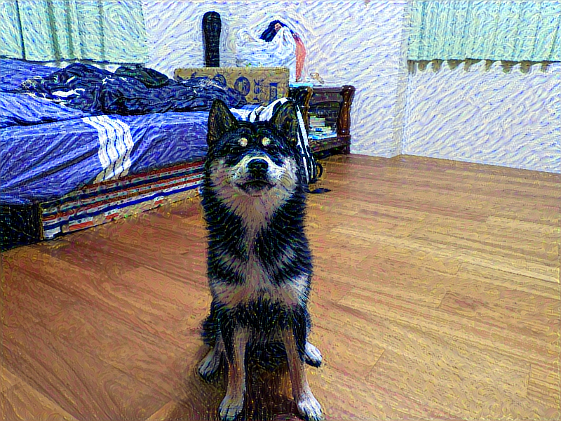
藝術風格轉換的主要目的是將一張參考圖片(就是一張名畫)的風格(style)，套用到另一張普通的原始圖片上，最後生成的圖片既能保留原始圖片的大致內容，又能展現出名畫的風格。這裡得風格，狹義的定義，是指名畫中的的紋理、色彩、視覺模式等等。比如紋理有個特點是和所在位置無關，基於這個特點，只要是和位置無關的統計信息，都可以試著來表示紋理的特徵。而原始圖片的內容 (content)，則指的是圖片的宏觀構造。

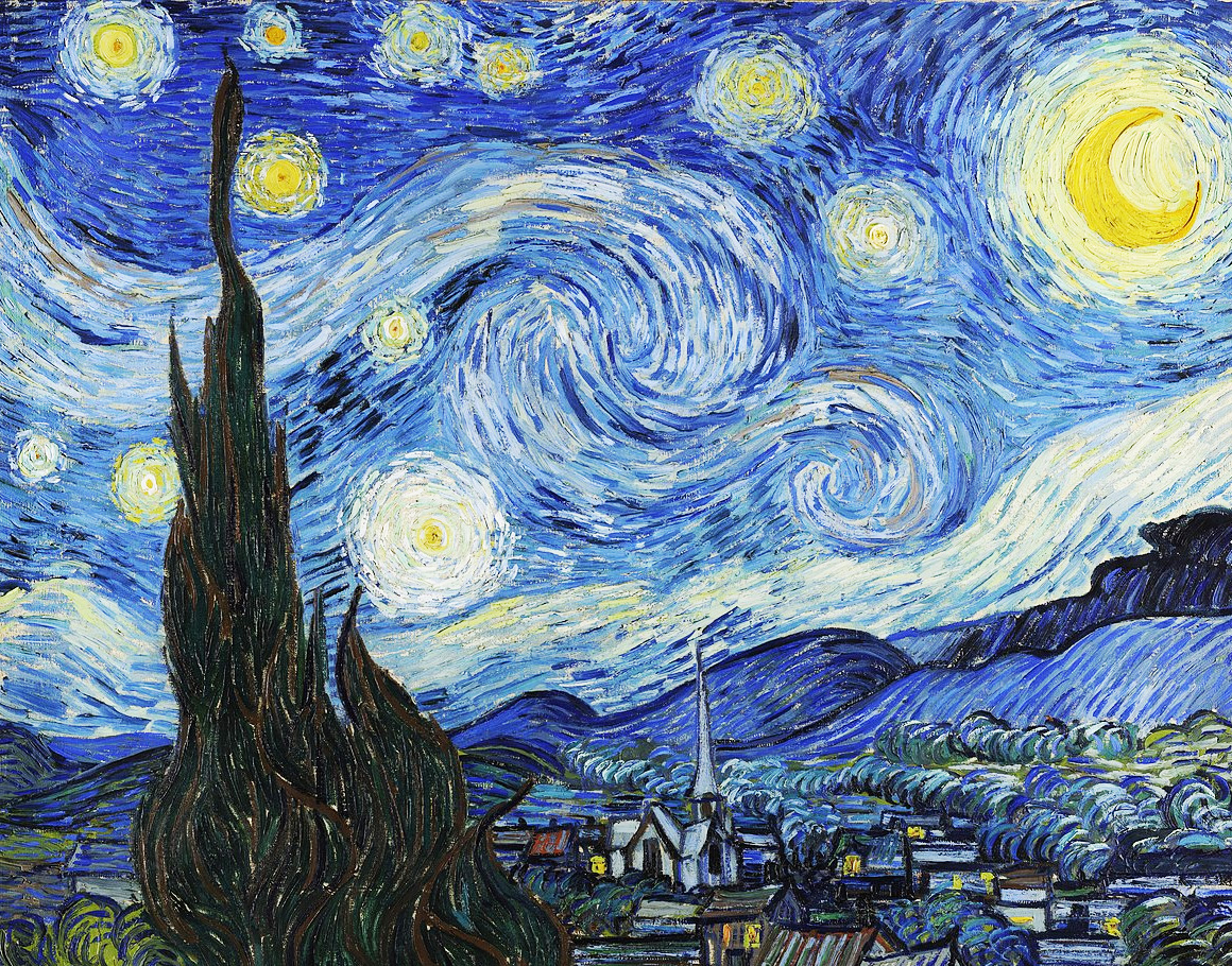
本人是看不出這到底有什麼價值啦，也實在看不出底下的風格照到底是在有名什麼意思。不過本人猜想能讓專家看不出這是電腦繪製，而且會被誤會成是人工繪製的，那就是有價值的 “真品” 吧。

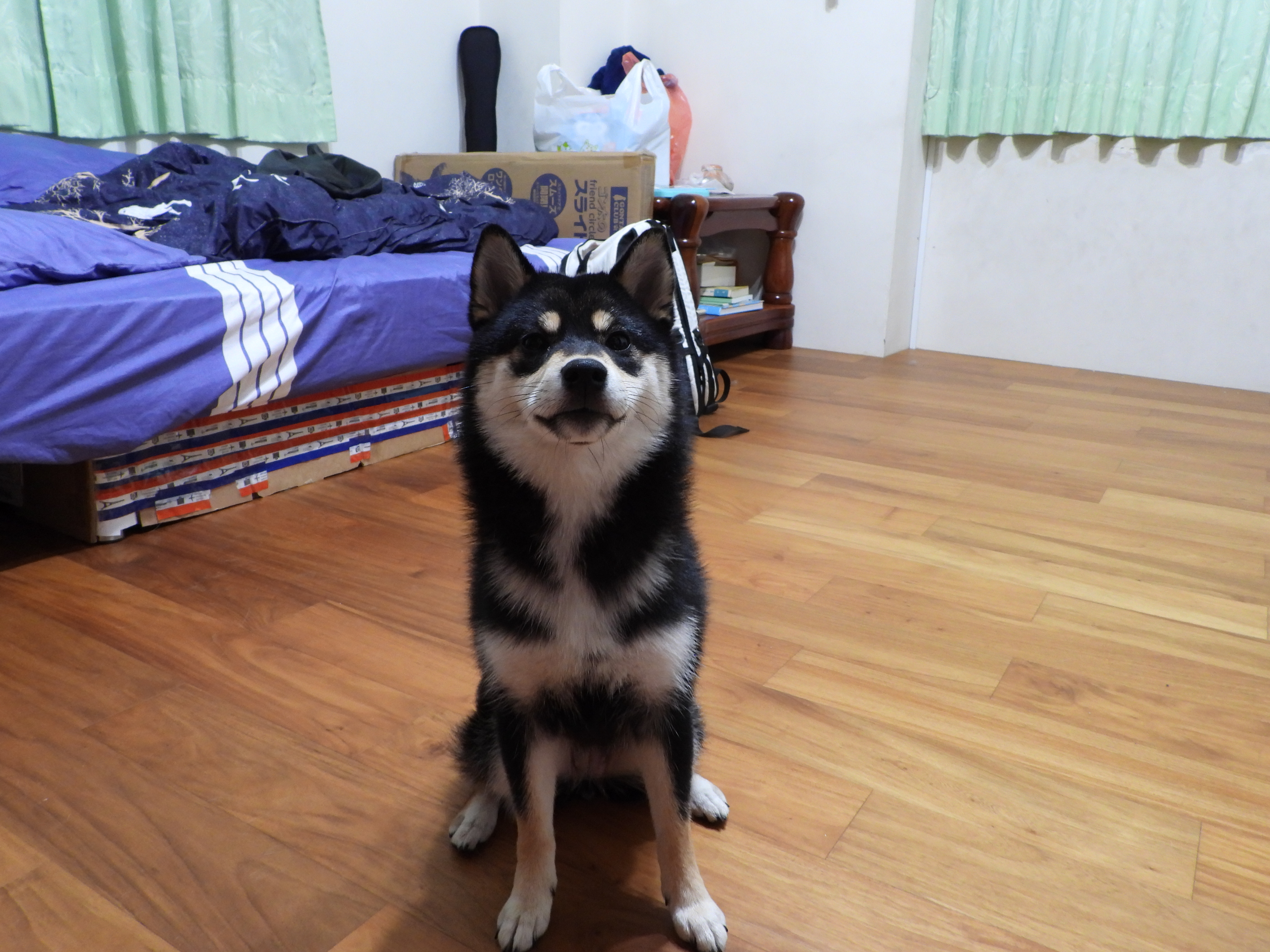
底下是本範例產生的結果

原始圖 :

風格照 :

合成圖 :

硬体限制

顯卡內存如果是 12G 的話，只能把圖片縮小到 1500 *1125 的解析度，超出這個範圍就會出現 OOM 的錯誤。

向量內積

二個向量相對應的位置相乘後求總和。以數學公式定義如下

$(a=\begin{bmatrix}a_{1}, a_{2}, a_{3}, …., a_{n}\end{bmatrix})$

$(b=\begin{bmatrix}b_{1}, b_{2}, b_{3}, …., b_{n}\end{bmatrix})$

$(a\cdot b = a_{1}b_{1} + a_{2}b_{2} + a_{3}b_{3} + …. +a_{n}b_{n})$

向量內積的作用是在判斷二向量之間的夾角和方向關係。

$(a\cdot b>0)$ : 方向大致相同，夾角在$(0^{\circ} \sim 90^{\circ})$之間

$(a\cdot b=0)$ : 正交，相互垂直

$(a\cdot b<0)$ : 方向基本相反，夾角在$(90^{\circ} \sim 180^{\circ})$之間

格拉姆矩陣 Gram Matrix

格拉姆矩陣定義如下

$(G(x_{1},x_{2},x_{2},…,x_{n}) = \begin{bmatrix}
(x_{1}x_{1})&(x_{1}x_{2})&…&(x_{1}x_{n})\\
(x_{2}x_{1})&(x_{2}x_{2})&…&(x_{2}x_{n})\\
… & … & … & \\
(x_{n}x_{1})&(x_{n}x_{2})&…&(x_{n}x_{n})\\
\end{bmatrix})$

底下的代碼，使用 np.outer(a,a) 即可算出格拉姆的結果

import numpy as np
a=np.array([1,2,3,4,5])
print(np.outer(a,a))
結果:
[[ 1  2  3  4  5]
 [ 2  4  6  8 10]
 [ 3  6  9 12 15]
 [ 4  8 12 16 20]
 [ 5 10 15 20 25]]

上述先取得 “1” , 然後跟 [1,2,3,4,5]相乘產生第一列的結果，再取 “2” , 然後跟 [1,2,3,4,5] 相乘而產生第二列的結果，依此類推。

二維格拉姆陣列

二維陣列，比如 (3，5) 的 a 陣列，需先轉置成 (5, 3) 的 b 二維陣列

接著把 b 陣列扁平化成 [1,6, 11, 2, 7, 12, 3, 8, 13, 4, 9, 14, 5, 10, 15]
取 a 的第一個值 “1” 跟 b 相乘，形成第一列
取 a 的第二個值 “2” 跟 b 相乘，形成第二列
其餘以此類推

最後的結果，是 (3*5，3*5) = (15，15) 的二維陣列

import numpy as np
a = np.array([[1,2,3,4,5], [6, 7, 8, 9, 10], [11,12,13,14,15]])
#b = np.transpose(a)
b = a.T
print("a 陣列如下")
print(a)
print("b 陣列如下")
print(b)
print("格拉姆陣列如下")
print(np.outer(a,b))
結果 :
a 陣列如下
[[ 1  2  3  4  5]
 [ 6  7  8  9 10]
 [11 12 13 14 15]]
b 陣列如下
[[ 1  6 11]
 [ 2  7 12]
 [ 3  8 13]
 [ 4  9 14]
 [ 5 10 15]]
格拉姆陣列如下
[[  1   6  11   2   7  12   3   8  13   4   9  14   5  10  15]
 [  2  12  22   4  14  24   6  16  26   8  18  28  10  20  30]
 [  3  18  33   6  21  36   9  24  39  12  27  42  15  30  45]
 [  4  24  44   8  28  48  12  32  52  16  36  56  20  40  60]
 [  5  30  55  10  35  60  15  40  65  20  45  70  25  50  75]
 [  6  36  66  12  42  72  18  48  78  24  54  84  30  60  90]
 [  7  42  77  14  49  84  21  56  91  28  63  98  35  70 105]
 [  8  48  88  16  56  96  24  64 104  32  72 112  40  80 120]
 [  9  54  99  18  63 108  27  72 117  36  81 126  45  90 135]
 [ 10  60 110  20  70 120  30  80 130  40  90 140  50 100 150]
 [ 11  66 121  22  77 132  33  88 143  44  99 154  55 110 165]
 [ 12  72 132  24  84 144  36  96 156  48 108 168  60 120 180]
 [ 13  78 143  26  91 156  39 104 169  52 117 182  65 130 195]
 [ 14  84 154  28  98 168  42 112 182  56 126 196  70 140 210]
 [ 15  90 165  30 105 180  45 120 195  60 135 210  75 150 225]]

三維格拉姆

歹勢喔，沒有三維格接姆，最多只有二維。所以必需將多維陣列轉成二維陣列，再計算格拉姆。

變異數(Variance)與標準差(standard deviation)

由以前的說明，標準差是將 (所有數-平均值)平方總和/總數，再開根號，數學公式如下。

$(\sqrt{\frac{1}{n}\sum (x_{i}-mean)^{2}})$

那麼變異數又是什麼? 就是上述計算時，不開根號。

$(\frac{1}{n}\sum (x_{i}-mean)^{2})$

也就是說，標準差就是變異數的開根號。由如下代碼可以驗証

import numpy as np
np.random.seed(1)
a=np.random.randint(1,100,10)
mean=a.mean()
sum=0
for i in a:
    sum+=(i-mean)**2
print("手動變異數",sum/10)
print("手動標準差",(sum/10)**0.5)
print("np 變異數",np.var(a))
print("np 標準差",np.std(a))

結果:
手動變異數 933.2
手動標準差 30.548322376196047
np 變異數 933.2
np 標準差 30.548322376196047

圖片應用

上述講了一大堆數學的計算方法，實在是搞不懂要幹嘛，所以底下用圖片的方式來說明其運用。

讀取圖片後，需先把圖片縮小到 800*600 像素左右，如果圖片過大，產生的格拉姆陣列會超級大的，會產生記憶体不足的問題。

由 cv2 讀取的格式，是 [h, w, c] 的三維陣列，h是高度，w是寬度，c 是 channel (BGR，固定為 3)。所以必需使用 np.transport(img, (2, 0, 1)) 把 chanel 拉到最前面的維度，變成 [c, h, w] 的三維陣列，然後再用 np.reshape(3, -1) 變成 [3, h*w] 的二維陣列。經此轉換後，會變成第一列為每點藍色值偏平化，第二列為綠色值偏平化，第三列為紅色值偏平化。

[[藍1, 藍2, 藍3, 藍4, ……藍n],
[綠1, 綠2, 綠3, 綠4, ……綠n],
[紅1, 紅2, 紅3, 紅4, ……紅n]]

最後產生的格拉姆二維陣列為 [3*h*w, 3*h*w]。

import numpy as np
import cv2
base_path='./images/input6.jpg'
img = cv2.imdecode(np.fromfile(base_path, dtype=np.uint8), cv2.IMREAD_UNCHANGED)
original_height,original_width=img.shape[:2]
height=100
width= round(original_width * height / original_height)
print(f'圖片 高*寬: {height}*{width}')
img = cv2.resize(img, (width, height))
img = cv2.cvtColor(img, cv2.COLOR_BGR2RGB)

#將[h, w, c] 轉成 [c, h, w]
img=np.transpose(img,(2,0,1))
a=np.reshape(img, (3, -1)).astype(np.int32)
b=np.transpose(a, (1, 0)).astype(np.int32)
c=np.outer(a,b)
print("格拉姆 shape : ",c.shape)
print(c)
結果 :
圖片 高*寬: 100*133
格拉姆 shape : (39900, 39900)
[[33124 36218 39676 ... 32032 32214 32942]
[32760 35820 39240 ... 31680 31860 32580]
[33670 36815 40330 ... 32560 32745 33485]
...
[33670 36815 40330 ... 32560 32745 33485]
[29848 32636 35752 ... 28864 29028 29684]
[32942 36019 39458 ... 31856 32037 32761]]

格拉姆是在取得每個特徵跟其它特徵之間的關聯性。這個關聯性可以想成是在取得某個空間要使用的紋理，這樣相同的紋理就會重複出在不同的位置。

風格轉換步驟

底下是風格轉換的步驟。一開始合成圖跟原始圖是一模一樣的。

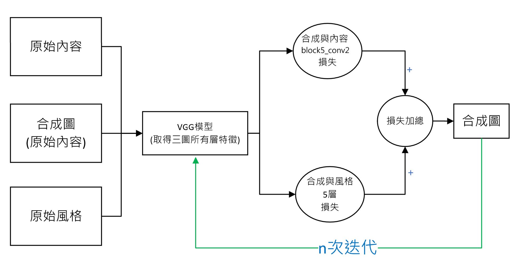
公式總覽

底下的觀念及代碼非常的複雜，所以只要記得 Gatys 等人所定義的方式即可。等這些定義記熟了之後，再慢慢的去探討相關的理論。

一開始，合成圖與原始內容圖一模一樣。
計算原始內容與合成圖 “block5_conv2” 特徵損失 + 風格圖及合成圖 “block1_conv1”, “block2_conv1”, “block3_conv1”, “block4_conv1”, “block5_conv1” 5 層特徵的格拉姆損失。
計算上述損失函數的梯度下降。
解開合成圖查看結果。
重複 2~4 步驟 4000次。

上述第 4 步驟點，並不是每一次都要解開圖片觀看，否則會很慢。所以可以每 100 個步驟再解開一次。

VGG19 Block

vgg19 模型總共有 5個block, 每個 block由2~4個捲積層組成。較低階的block(比如 block1) 所取得的特徵數較少，比如 block1只有64個特徵，通常是取得顏色，邊緣等特徵。較高階的block, 比如block5 加深了特徵的截取，所以特徵數較多，比如block5可達512種特徵，這通常代表著元素的組成單位，比如點線弧等特徵。

model = applications.vgg19.VGG19(weights="imagenet", include_top=False)
outputs_dict = dict([(layer.name, layer.output) for layer in model.layers])
for i, layer in enumerate(model.layers):
    print(i+1, layer.name)
結果:
1 input_1
2 block1_conv1
3 block1_conv2
4 block1_pool
5 block2_conv1
6 block2_conv2
7 block2_pool
8 block3_conv1
9 block3_conv2
10 block3_conv3
11 block3_conv4
12 block3_pool
13 block4_conv1
14 block4_conv2
15 block4_conv3
16 block4_conv4
17 block4_pool
18 block5_conv1
19 block5_conv2
20 block5_conv3
21 block5_conv4
22 block5_pool

原理

利用損失函數的組合產生合成圖，整体的函數為

$(Loss(C)= \sum (B_{i}^{b5c2}-C_{i}^{b5c2})^2 +)$

$(\sum (G(S_{i}^{b1c1}-C_{i}^{b1c1})^2+\sum (G(S_{i}^{b2c1}-C_{i}^{b2c1})^2+ )$

$(\sum (G(S_{i}^{b3c1}-C_{i}^{b3c1})^2+\sum (G(S_{i}^{b4c1}-C_{i}^{b4c1})^2+ )$

$(\sum (G(S_{i}^{b5c1}-C_{i}^{b5c1})^2)$

vgg19 模型總共

原始圖與合成圖損失

合成圖一開始跟原始圖一樣。每一次迭代，都要盡量與原始圖一樣，所以只需高階 block5_conv2 捲積層取得最為詳細的特徵。所以只要計算 block5_conv2 的損失函數即可。損失函數為 (原始內容 – 合成圖) 的平方總和。最後因為損失值過大，所以要乘上一個權重，目前我們定為content_weight = 2.5e-8

loss = loss + content_weight * tf.reduce_sum(tf.square(combination_feature - base_feature))

風格圖與合成圖損失

風格圖與合成圖的組合，需將 block1~5 的 conv1 5層作損失函數加總，也就是要提取風格照的邊緣，紋理等所有的特徵。每層加總前，需將風格圖與合成照改成格拉姆矩陣 s 及 c，然後將 (s-c) 平方，再除以 (4*(channels**2)*(size**2)) 縮小損失，再作加總。最後將這5層的損失相加。

使用格拉姆矩陣的目地，是在取得各個特徵之間的關聯性，這此關聯性代表著該空間比例下所辨識出的紋理外觀，這個風格照的特定紋理就會重複出現在合成照的不同地方。如果不使用格拉姆矩陣的話，就只是把整張風格照模糊化然後套到合成照中。

def style_loss(style_feature, combination_feature):
    s = gram_matrix(style_feature)
    c = gram_matrix(combination_feature)
    channels = 3
    size = height * width

    #(4.0*(channels ** 2) * (size **2)) 為官網建議，可以自已調整看看
    return tf.reduce_sum(tf.square(s - c)) / (4.0 * (channels ** 2) * (size ** 2))

for layer_name in style_layer_names:
    style_feature = style_features[layer_name]
    combination_feature=combination_features[layer_name]
    loss = style_loss(
        style_feature, combination_feature)
    total_loss += (style_weight / len(style_layer_names)) * loss

preprocess_input

keras 的 preprocess_input 會先把 RGB (224,224,3) 轉成 (1, 224,224,3) 維，然後將每個點的值減去平均值，讓每個值分佈在 0 的左右二邊(有正有負)，以適用於 ResNet50 的要求。

完整代碼

#pip install tensorflow opencv-python matplotlib
import os
os.environ['TF_CPP_MIN_LOG_LEVEL']='2'
import shutil
import keras
import numpy as np
from keras.src.applications.vgg19 import VGG19, preprocess_input
from keras.src.optimizers import SGD
from MahalSdk.cv import cv
import cv2
import tensorflow as tf
import pylab as plt
def deprocess_image(img):
    # img 為(1, 600, 800, 3) 4維度, 需改成 (600,800,3) 3維度
    img=np.reshape(img, (height, width, 3))[:,:,::-1].copy()
    #底下是將亮度調亮
    img[:, :, 0] += 123.68
    img[:, :, 1] += 116.779
    img[:, :, 2] += 103.939

    #將小於 0 的值變為 0，超出 255 的值，改為255
    img = np.clip(img, 0, 255).astype(np.uint8)
    return img
#加入全變異損失，會有較小的變化，也可以不加
def total_variation_loss(x):
    a = tf.square(
        x[:, : height - 1, : width - 1, :] - x[:, 1:, : width - 1, :]
    )
    b = tf.square(
        x[:, : height - 1, : width - 1, :] - x[:, : height - 1, 1:, :]
    )
    return tf.reduce_sum(tf.pow(a + b, 1.25))
def gram_matrix(x):
    x=tf.reshape(x, (x.shape[1], x.shape[2], x.shape[3]))
    x=tf.transpose(x, (2, 0, 1))
    features=tf.reshape(x, (tf.shape(x)[0], -1))
    gram=tf.matmul(features, tf.transpose(features))
    return gram
def content_loss(base_feature, combination_feature):
    return tf.reduce_sum(
        tf.square(base_feature - combination_feature)
    ) * content_weight
def style_loss(style_feature, combination_feature):
    s=gram_matrix(style_feature)
    c=gram_matrix(combination_feature)
    channels=3
    size=width*height
    # (4.0*(channels ** 2) * (size **2)) 為官網建議，可以自已調整看看
    return tf.reduce_sum(tf.square(s-c))/(4*(channels**2)*(size**2)) * style_weight
#@tf.function
def compute_grads(combination_img, base_img, style_img):
    base_features = model(base_img)
    base_feature = base_features[content_layer_name]
    style_featuers=model(style_img)
    with tf.GradientTape() as tape:
        #一定要寫在 with 區塊中
        total_loss = tf.zeros(shape=())
        combination_features = model(combination_img)
        combination_feature=combination_features[content_layer_name]
        total_loss += content_loss(base_feature, combination_feature)
        for layer in style_layer_names:
            style_feature=style_featuers[layer]
            combination_feaure=combination_features[layer]
            #底下需先轉成格拉姆再計算 loss
            total_loss+=style_loss(style_feature, combination_feaure)
    grads=tape.gradient(total_loss, combination_img)
    return grads
model=VGG19(weights='imagenet', include_top=False)
outputs=dict([(layer.name, layer.output) for layer in model.layers])
model=keras.Model(inputs=model.input, outputs=outputs)
content_layer_name='block5_conv2'
style_layer_names=[
    'block1_conv1',
    'block2_conv1',
    'block3_conv1',
    'block4_conv1',
    'block5_conv1',
]
total_variation_weight=1e-6
style_weight=1e-6/len(style_layer_names)
content_weight=2.5e-8
base_img=cv.resize(
    cv.read("draw_1.jpg")[:,:,::-1].copy(),
    width=1500
)
height, width, _ = base_img.shape
print(height, width)
base_img=preprocess_input(np.expand_dims(base_img, axis=0))

style_img=cv2.resize(
    cv.read("starry_night.jpg")[:,:,::-1].copy(),
    (width, height),
    interpolation=cv2.INTER_LINEAR)
style_img=preprocess_input(np.expand_dims(style_img, axis=0))
combination_img=tf.Variable(base_img)
epochs=4001
optimizer=SGD(
    keras.optimizers.schedules.ExponentialDecay(
        initial_learning_rate=100.0,
        decay_steps=100,
        decay_rate=0.96
    )
)
output_path="./output"
if os.path.exists(output_path):
    shutil.rmtree(output_path)
os.mkdir(output_path)
fig, ax=plt.subplots()
for i in range(epochs):
    grads=compute_grads(
        combination_img,base_img, style_img
    )
    optimizer.apply_gradients([(grads, combination_img)])
    img=deprocess_image(combination_img.numpy())
    if i % 100==0:
        file=os.path.join(output_path, f'combination_epoch{i}.jpg')
        pil = Image.fromarray(img)
        pil.save(file)
        #keras.utils.save_img(file, img)
        ax.clear()
        ax.axis("off")
        ax.imshow(img)
        plt.pause(0.01)
    print(f'epoch : {i}')
plt.show()

Epochs

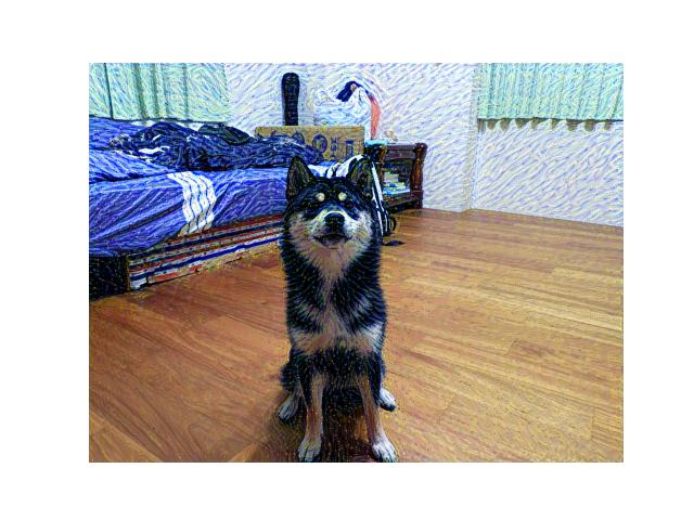
上述如果將 Epochs 改到 10000，結果跟 4000 差不多，風格紋理並不會覆蓋掉原始狗狗的圖片，如下圖所示

colab版本

在 colab 裏執行，無法使用 plt 持續更新，需使用 cv2_imshow 才能更新圖片，完整代碼如下

#pip install tensorflow opencv-python matplotlib
#先將 draw_1.jpg 與 starry_night.jpg copy 到雲端硬碟的 pictures 資料夾
from google.colab import drive
from google.colab.patches import cv2_imshow
import os.path
import shutil
import keras
import numpy as np
drive.mount('/data')
pic_path="/data/MyDrive/pictures"
sdk_path="/data/MyDrive/sdk/"
import sys
sys.path.append(sdk_path)
from cv import cv
from keras.src.applications.vgg19 import VGG19, preprocess_input
from keras.src.optimizers import SGD
import cv2
import tensorflow as tf
import pylab as plt
def deprocess_image(img):
    # img 為(1, 600, 800, 3) 4維度, 需改成 (600,800,3) 3維度
    #img=img.reshape((height, width, 3))[:,:,::-1].copy()
    img=np.reshape(img, (height, width, 3))[:,:,::-1].copy()
    #底下是將亮度調亮
    img[:, :, 0] += 123.68
    img[:, :, 1] += 116.779
    img[:, :, 2] += 103.939

    #將小於 0 的值變為 0，超出 255 的值，改為255
    img = np.clip(img, 0, 255).astype(np.uint8)
    return img
#加入全變異損失，會有較小的變化，也可以不加
def total_variation_loss(x):
    a = tf.square(
        x[:, : height - 1, : width - 1, :] - x[:, 1:, : width - 1, :]
    )
    b = tf.square(
        x[:, : height - 1, : width - 1, :] - x[:, : height - 1, 1:, :]
    )
    return tf.reduce_sum(tf.pow(a + b, 1.25))
def gram_matrix(x):
    x=tf.reshape(x, (x.shape[1], x.shape[2], x.shape[3]))
    x=tf.transpose(x, (2, 0, 1))
    features=tf.reshape(x, (tf.shape(x)[0], -1))
    gram=tf.matmul(features, tf.transpose(features))
    return gram
def content_loss(base_feature, combination_feature):
    return tf.reduce_sum(
        tf.square(base_feature - combination_feature)
    ) * content_weight
def style_loss(style_feature, combination_feature):
    s=gram_matrix(style_feature)
    c=gram_matrix(combination_feature)
    channels=3
    size=width*height
    # (4.0*(channels ** 2) * (size **2)) 為官網建議，可以自已調整看看
    return tf.reduce_sum(tf.square(s-c))/(4*(channels**2)*(size**2)) * style_weight
#@tf.function
def compute_grads(combination_img, base_img, style_img):
    base_features = model(base_img)
    base_feature = base_features[content_layer_name]
    style_featuers=model(style_img)
    with tf.GradientTape() as tape:
        #一定要寫在 with 區塊中
        total_loss = tf.zeros(shape=())
        combination_features = model(combination_img)
        combination_feature=combination_features[content_layer_name]
        total_loss += content_loss(base_feature, combination_feature)
        for layer in style_layer_names:
            style_feature=style_featuers[layer]
            combination_feaure=combination_features[layer]
            #底下需先轉成格拉姆再計算 loss
            total_loss+=style_loss(style_feature, combination_feaure)
    grads=tape.gradient(total_loss, combination_img)
    return grads
model=VGG19(weights='imagenet', include_top=False)
outputs=dict([(layer.name, layer.output) for layer in model.layers])
model=keras.Model(inputs=model.input, outputs=outputs)
content_layer_name='block5_conv2'
style_layer_names=[
    'block1_conv1',
    'block2_conv1',
    'block3_conv1',
    'block4_conv1',
    'block5_conv1',
]
total_variation_weight=1e-6
style_weight=1e-6/len(style_layer_names)
content_weight=2.5e-8
base_img=cv.resize(
    cv.read(os.path.join(pic_path,"draw_1.jpg"))[:,:,::-1].copy(),
    width=1500
)
height, width, _ = base_img.shape
print(height, width)
base_img=preprocess_input(np.expand_dims(base_img, axis=0))

style_img=cv2.resize(
    cv.read(os.path.join(pic_path,"starry_night.jpg"))[:,:,::-1].copy(),
    (width, height),
    interpolation=cv2.INTER_LINEAR)
style_img=preprocess_input(np.expand_dims(style_img, axis=0))
combination_img=tf.Variable(base_img)
epochs=4001
optimizer=SGD(
    keras.optimizers.schedules.ExponentialDecay(
        initial_learning_rate=100.0,
        decay_steps=100,
        decay_rate=0.96
    )
)
output_path="./output"
if os.path.exists(os.path.join(pic_path,output_path)):
    shutil.rmtree(os.path.join(pic_path,output_path))
os.mkdir(os.path.join(pic_path,output_path))
#fig, ax=plt.subplots()
for i in range(epochs):
    grads=compute_grads(
        combination_img,
        base_img,
        style_img
    )
    optimizer.apply_gradients([(grads, combination_img)])
    img=deprocess_image(combination_img)
    if i %100==0:
        file=os.path.join(pic_path, output_path, f'combination_epoch{i}.jpg')
        pil = Image.fromarray(img)
        pil.save(file)
        keras.utils.save_img(file,img)
        cv2_imshow(cv2.cvtColor(img, cv2.COLOR_RGB2BGR))
        cv2.waitKey(1)#不等待的話，無法顯示圖片
    print(f"epoch : {i}")

參考

https://edge.aif.tw/booklist-deep-learning-with-python/

官網 : https://colab.research.google.com/drive/1fxaotuK2U_I1H82i4j6TftQ3qGtGOkcl?usp=sharing#scrollTo=MroM_ZjvV-D0

https://www.cnblogs.com/yifanrensheng/p/12547660.html

神經網路風格轉換

神經網路風格轉換

硬体限制

相關演算法

向量內積

格拉姆矩陣 Gram Matrix

二維格拉姆陣列

三維格拉姆

變異數(Variance)與標準差(standard deviation)

圖片應用

風格轉換步驟

公式總覽

VGG19 Block

原理

原始圖與合成圖損失

風格圖與合成圖損失

preprocess_input

完整代碼

Epochs

colab版本

參考

發佈留言